Lecture 1: Introduction to Non-Euclidean Data Analysis
Why Euclidean spaces are not enough
1 Learning Goals
By the end of this lecture, learners should be able to:
- Identify algebraic and geometric features of \(\mathbb{R}^p\) that classical statistics relies on.
- Define Euclidean and non-Euclidean spaces precisely.
- Describe concrete examples of non-Euclidean data spaces: trees, SPD matrices, spheres, simplices, and Wasserstein spaces.
- Contrast the general metric-space approach with the Riemannian-manifold approach to non-Euclidean statistics.
2 Euclidean Spaces: What and Why
Classical statistics is largely formulated for data taking values in Euclidean spaces such as \(\mathbb{R}^p\). Euclidean spaces come with a rich collection of algebraic and geometric structures: points can be added and subtracted, scalar multiplication is available, inner products induce norms and angles, and straight lines provide canonical interpolations between observations. These structures make familiar statistical operations possible. Sample means, covariance matrices, principal component analysis, linear regression, and Gaussian models all rely, either explicitly or implicitly, on the idea that data behave like vectors.
Consider the space \(\mathbb{R}^p\), endowed with the standard inner product \(\langle x, y \rangle = x^\top y\) for \(x, y \in \mathbb{R}^p\). This inner product induces the Euclidean norm \(\|x\|_2 = \langle x, x \rangle^{1/2}\) and the distance
\[ d(x, y) = \|x - y\|_2. \]
An inner product on a real vector space \(V\) is a function \(\langle\cdot,\cdot\rangle : V \times V \to \mathbb{R}\) satisfying the following axioms for all \(u, v, w \in V\) and \(a, b \in \mathbb{R}\):
- Symmetry: \(\langle u, v \rangle = \langle v, u \rangle\)
- Linearity in the first argument: \(\langle a u + b v, w \rangle = a\langle u, w \rangle + b\langle v, w \rangle\)
- Positive-definiteness: \(\langle u, u \rangle \ge 0\), with equality if and only if \(u = 0\)
From these axioms, an inner product induces a norm \(\|u\| := \sqrt{\langle u, u \rangle}\) and a distance \(d(u, v) := \|u - v\|\). Moreover, it defines the notion of angle between nonzero vectors via \(\cos\theta = \langle u, v \rangle / (\|u\|\|v\|)\), and in particular orthogonality: \(u \perp v\) when \(\langle u, v \rangle = 0\).
Key examples:
Standard (dot) inner product on \(\mathbb{R}^p\): \(\langle x, y \rangle = \sum_{i=1}^p x_i y_i = x^\top y\). This is the familiar Euclidean inner product that underpins least squares, PCA, and virtually all of classical multivariate analysis.
Frobenius inner product on matrices: For \(A, B \in \mathbb{R}^{m \times n}\), \(\langle A, B \rangle_F = \operatorname{tr}(A^\top B) = \sum_{i=1}^m \sum_{j=1}^n a_{ij} b_{ij}\). This turns the space of matrices into a Euclidean space of dimension \(mn\). The induced Frobenius norm \(\|A\|_F = \sqrt{\operatorname{tr}(A^\top A)}\) measures the entrywise magnitude of a matrix.
\(L^2\) inner product on functions: For square-integrable functions \(f, g\) on \([0,1]\), \(\langle f, g \rangle = \int_0^1 f(t) g(t)\,dt\). This inner product underpins functional data analysis and arises naturally in the one-dimensional Wasserstein geometry via quantile functions.
Many non-Euclidean spaces lack an inner product (or a norm induced by one). The parallelogram law provides an operational test: a norm comes from an inner product if and only if it satisfies \(\|u+v\|^2 + \|u-v\|^2 = 2\|u\|^2 + 2\|v\|^2\) for all \(u, v\). This is the content of the von Neumann–Jordan theorem, and it explains why \(\ell_1\), \(\ell_\infty\), and many other norms do not admit inner products.
To clarify the meaning of non-Euclidean space, it is convenient to specify precisely what is meant by a Euclidean space. \((\mathbb{R}^p, \langle\cdot,\cdot\rangle)\) is an example of Euclidean space, but the definition of Euclidean space is more general.
Definition 1 A Euclidean space is a finite-dimensional normed space isometrically isomorphic to \((\mathbb{R}^p, \langle\cdot,\cdot\rangle)\) for some integer \(p \ge 1\).
Example 1 The space of \(p \times p\) symmetric matrices with the Frobenius inner product \(\langle A, B \rangle = \operatorname{tr}(A^\top B)\) is a Euclidean space.
Definition 2 In this note, a non-Euclidean space is any space that is not isometrically isomorphic to \((\mathbb{R}^p, \langle\cdot,\cdot\rangle)\) for any \(p \ge 1\).
A normed vector space is a pair \((V, \|\cdot\|)\) where \(V\) is a real vector space and \(\|\cdot\| : V \to [0,\infty)\) is a function satisfying:
- Positive-definiteness: \(\|x\| = 0\) iff \(x = 0\);
- Absolute homogeneity: \(\|ax\| = |a|\,\|x\|\) for all \(a \in \mathbb{R}\);
- Triangle inequality: \(\|x + y\| \le \|x\| + \|y\|\).
A norm induces a metric \(d(x,y) = \|x - y\|\). An isometrical isomorphism (or linear isometry) between two normed spaces \((V, \|\cdot\|_V)\) and \((W, \|\cdot\|_W)\) is a linear map \(T : V \to W\) that is bijective and distance-preserving: \(\|T(v)\|_W = \|v\|_V\) for all \(v \in V\). If such a map exists, the spaces are said to be isometrically isomorphic.
A Euclidean space is defined as a finite-dimensional normed space that is isometrically isomorphic to \((\mathbb{R}^p, \|\cdot\|_2)\) for some \(p\ge 1\). The Mazur–Ulam theorem ensures that any surjective isometry between real normed spaces is affine, so metric isometry plus vector-space structure automatically forces linearity in this context.
The following algebraic and geometric features of \(\mathbb{R}^p\) are used repeatedly in statistics.
Vector space structure — points can be added, subtracted, and rescaled, which facilitates the definition of linear combinations, expectations, and centered observations.
Inner product and orthogonality — angles, orthogonality, and orthogonal decompositions are available, underpinning least-squares methods, covariance analysis, and principal component analysis.
Norm and metric structure — the Euclidean norm yields a translation-invariant distance, allowing variation to be measured through squared distances, variances, and second moments.
Affine and geodesic structure — straight lines \(t \mapsto (1-t)x + ty\) are globally defined and provide the canonical interpolations between observations; they are also the geodesics of the space.
Convexity and projections — convex combinations remain in the space, convex sets behave well, and closed convex sets admit unique orthogonal projections, which are fundamental in optimization and constrained estimation.
Global coordinates and linear operators — a single coordinate system covers the whole space, and linear transformations can be represented by matrices, making multivariate analysis globally coherent.
Flat homogeneous geometry — the space has zero curvature and no preferred direction, so the same statistical procedures can be transported consistently across the sample space.
Finite dimension — the dimension of a Euclidean space is finite, which guarantees that all norms are equivalent, compactness and continuity arguments are tractable on bounded sets, and matrix-based descriptions of covariance, regression, and spectral decompositions remain available. In high-dimensional statistics, the dimension is allowed to diverge with the sample size but is still finite.
3 Ways to Fail Being Euclidean
Many modern data objects are not naturally represented by unconstrained vectors in a Euclidean space. A space may fail to be Euclidean at different structural levels:
| Level | Failure | Example |
|---|---|---|
| 1 | Not a metric space | A bare set \(\mathcal{M}\) with no distance |
| 2 | Metric space, but not a vector space | \(\mathbb{S}^2\) with geodesic distance |
| 3 | Vector space, metric not norm-induced | \(\mathbb{R}\) with \(d(x,y) = \min\{1, |x-y|\}\) |
| 4 | Normed space, norm not inner-product | \((\mathbb{R}^2, \|\cdot\|_1)\) |
| 5 | Inner-product space, infinite-dimensional | \(\ell^2\) |
Let’s examine each level with concrete examples.
3.1 No Metric Structure
A bare set \(\mathcal{M}\) with no distance specified is not a metric space, hence cannot be Euclidean. This is the most extreme failure — without a distance, even basic notions like “closeness” or “convergence” are hard to define.
3.2 Metric Space Without Vector Structure
Example 2 The unit sphere
\[ \mathbb{S}^2 = \{x \in \mathbb{R}^3 : \|x\|_2 = 1\}, \]
equipped with the geodesic distance
\[ d_{\mathbb{S}^2}(x, y) = \arccos(\langle x, y \rangle), \]
is a metric space but not a vector space. Indeed, for \(x, y \in \mathbb{S}^2\), one generally has \(x + y \notin \mathbb{S}^2\), so the sphere is not closed under vector addition.
3.3 Vector Space With a Metric Not Induced by Any Norm
Example 3 The space \(\mathbb{R}\) is a vector space. Define a metric on it by
\[ d(x, y) = \min\{1, |x-y|\}, \qquad x, y \in \mathbb{R}. \]
This metric is not induced by any norm. Indeed, if a metric \(d\) comes from a norm, then it must satisfy the homogeneity property
\[ d(ax, ay) = |a|\, d(x, y), \qquad a \in \mathbb{R}. \]
However, for \(x = 0\), \(y = 1\), and \(a = 2\), we have
\[ d(0, 1) = 1, \qquad d(0, 2) = 1 \neq 2\,d(0, 1) = 2. \]
Hence \(d\) is not norm-induced.
3.4 Normed Space That Is Not Euclidean
Example 4 The space \((\mathbb{R}^2, \|\cdot\|_1)\), where
\[ \|(x, y)\|_1 = |x| + |y|, \]
is a normed vector space, but it is not Euclidean. Indeed, if a norm is induced by an inner product, then it must satisfy the parallelogram law
\[ \|u+v\|^2 + \|u-v\|^2 = 2\|u\|^2 + 2\|v\|^2 \qquad\text{for all } u, v. \]
Take \(u = (1, 0)\), \(v = (0, 1)\). Then
\[ \|u\|_1 = \|v\|_1 = 1, \qquad \|u+v\|_1 = \|u-v\|_1 = 2, \]
so
\[ \|u+v\|_1^2 + \|u-v\|_1^2 = 4 + 4 = 8, \]
whereas
\[ 2\|u\|_1^2 + 2\|v\|_1^2 = 2 + 2 = 4. \]
Thus the parallelogram law fails, and \(\|\cdot\|_1\) is not induced by any inner product. Therefore \((\mathbb{R}^2, \|\cdot\|_1)\) is not Euclidean.
3.5 Inner-Product Space That Is Not Euclidean
Example 5 The Hilbert space \(\ell^2 := \{x \in \mathbb{R}^\infty : \|x\|_2 < \infty\}\) with the inner product \(\langle x, y \rangle = \sum_{j=1}^\infty x_j y_j\) is an inner-product space, but it is infinite-dimensional, hence it is not linearly isometric to \(\mathbb{R}^p\) for any finite \(p\). Therefore, under our convention, \(\ell^2\) is non-Euclidean.
4 Metric Spaces
While technically speaking, non-Euclidean data may refer to data lying in a non-metric space, in this note we focus exclusively on data spaces endowed with a distance function.
Definition 3 A metric space is a pair \((\mathcal{M}, d)\) consisting of a set \(\mathcal{M}\) and a function \(d : \mathcal{M} \times \mathcal{M} \to [0, \infty)\) such that for all \(x, y, z \in \mathcal{M}\),
- (positivity) \(d(x, y) = 0\) if and only if \(x = y\);
- (symmetry) \(d(x, y) = d(y, x)\);
- (triangle inequality) \(d(x, z) \le d(x, y) + d(y, z)\).
The function \(d\) is called a metric or distance function on \(\mathcal{M}\).
5 Example: Tree-Valued Data (BHV Space)
Tree-valued observations arise in evolutionary biology, where posterior samples of phylogenetic trees encode uncertainty about species relationships, and in medical imaging, where airway, vascular, and dendritic branching systems are represented as anatomical trees (Billera et al. 2001; Feragen et al. 2013; Barden et al. 2013).
5.1 Construction
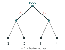
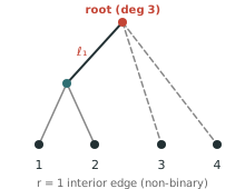
An \(m\)-tree is a tree with a distinguished vertex called the root and \(m\) leaves labeled \(1, \ldots, m\). We are mainly interested in rooted binary \(m\)-trees, where the root has degree \(2\) and every other internal vertex has degree \(3\), but nonbinary \(m\)-trees are needed to interpolate between different binary topologies.
A metric \(m\)-tree is an \(m\)-tree with positive lengths on all interior edges. Following Billera et al. (2001), the leaf edges are not included in the BHV coordinates, because allowing lengths on all leaf edges simply takes a Cartesian product with \(\mathbb{R}^m\) and does not change the essential geometry.
If \(T\) is a rooted metric \(m\)-tree with interior edges \(e_1, \ldots, e_r\) of lengths \(\ell_1, \ldots, \ell_r\), then the vector
\[ (\ell_1, \ldots, \ell_r) \in (0, \infty)^r \]
records the branch lengths of \(T\). If \(T\) is binary, then \(r = m-2\); otherwise \(r < m-2\). Boundary points in \([0, \infty)^r\) correspond to shrinking one or more interior edges to zero, thereby producing nonbinary \(m\)-trees.
5.2 Gluing the Orthants
The BHV space for rooted \(m\)-trees is obtained by taking one orthant \([0, \infty)^{m-2}\) for each combinatorial type of rooted binary \(m\)-tree and gluing orthants along common faces whenever the corresponding edge contractions produce the same nonbinary \(m\)-tree. Since the number of combinatorial types of rooted binary \(m\)-trees is
\[ (2m-3)!! = (2m-3) \cdot (2m-5) \cdots 5 \cdot 3 \cdot 1, \]
the space is assembled from \((2m-3)!!\) copies of \((m-2)\)-dimensional orthants.
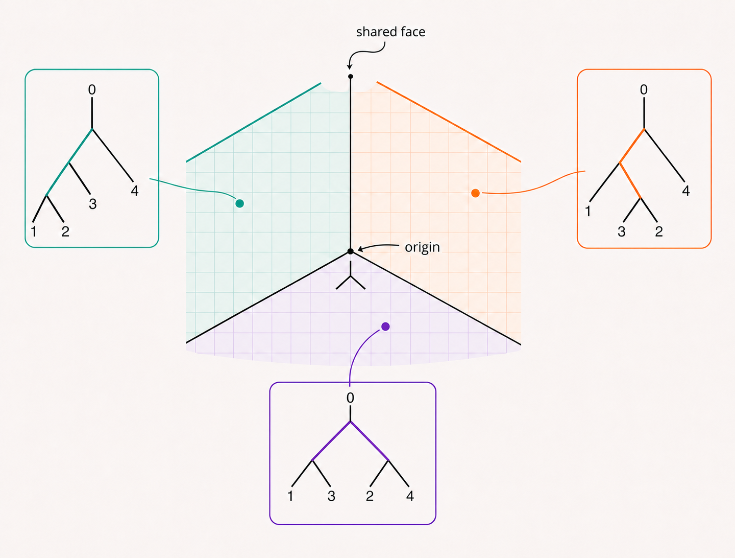
Figure: The BHV space is a cubical complex, where each orthant corresponds uniquely to a tree topology and the coordinates in each orthant parameterize its branch lengths.
5.3 Interactive Demo: Rooted Four-Leaf BHV Interpolation
The following demo specializes the construction above to a small local schematic inside the rooted \(m = 4\) case. Instead of drawing all \(15\) two-dimensional orthants, it shows three representative orthants arranged as three coordinate faces in a 3D view: \(O_1\) and \(O_2\) share one boundary axis, \(O_1\) and \(O_3\) share another, and \(O_2\) and \(O_3\) share a third. The path connecting the trees \(T_1\) and \(T_2\) are the shortest path between them in the BHV space.
5.4 The BHV Distance
If two trees \(T_1\) and \(T_2\) lie in the same orthant, their distance is the ordinary Euclidean distance between their edge-length vectors:
\[ d_{\mathrm{BHV}}(T_1, T_2) = \|\ell(T_1) - \ell(T_2)\|_2. \]
If they lie in different orthants, one joins them by a segmented path \(\gamma = \gamma_1 * \cdots * \gamma_R\), where each segment \(\gamma_r\) lies entirely in a single orthant, and defines the length of the path by summing the Euclidean lengths of the segments. The BHV distance is then the infimum over all such paths:
\[ d_{\mathrm{BHV}}(T_1, T_2) = \inf\{L(\gamma) : \gamma \text{ is a segmented path from } T_1 \text{ to } T_2\}. \]
5.5 Non-Euclidean Features
This space deviates from being Euclidean in several essential ways:
- It is not a vector space: rooted trees cannot be added or rescaled in a globally meaningful way.
- It is not a smooth manifold globally: nonbinary \(m\)-trees lie on singular strata where several orthants meet.
- It is piecewise Euclidean with different combinatorial tree shapes occupying different orthants.
Nevertheless, Billera et al. (2001) show that it has global nonpositive curvature, so geodesics and centroids behave much better than in a generic singular space.
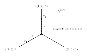
For \(m=3\) there are exactly three rooted binary \(3\)-trees, each having one interior edge, so \(\mathcal{T}^{\mathrm{BHV}}_3\) is obtained by gluing three rays at a common origin. The origin represents the rooted star tree with no interior edges, and the geodesic between trees on different rays passes through this origin; see the right panel of the figure above.
6 Example: Symmetric Positive-Definite (SPD) Matrices
Symmetric positive-definite (SPD) matrices arise as covariance matrices in multivariate analysis, diffusion tensors in magnetic resonance imaging, and covariance descriptors in computer vision (Pennec et al. 2006; Arsigny et al. 2006; Tuzel et al. 2006). The data space is
\[ \mathcal{S}_{++}^{m} = \{\Sigma \in \mathbb{R}^{m \times m} : \Sigma = \Sigma^\top \text{ and } x^\top \Sigma x > 0 \text{ for all } x \neq 0\}. \]
This is an open cone inside the vector space of symmetric matrices. It is not a linear subspace, since it is not closed under matrix addition or arbitrary scalar multiplication.
Brain functional connectivity. In resting-state fMRI, the pairwise Pearson correlations between \(m\) brain regions’ BOLD time series form an \(m \times m\) correlation matrix. Each subject or time window then corresponds to a point in \(\mathcal{S}_{++}^{m}\), making geodesic distances between such points natural tools for comparing connectivity patterns across individuals, cognitive states, or clinical conditions (Varoquaux et al. 2010; Pennec et al. 2006).
Portfolio risk. In quantitative finance, the covariance matrix of \(m\) asset returns is an important input to mean–variance portfolio optimisation. Provided no asset is a perfect linear combination of the others and the number of time periods exceeds \(m\), the sample covariance matrix is almost surely positive definite. Portfolios with different risk profiles map to different points in \(\mathcal{S}_{++}^{m}\); interpolation along geodesics in this space corresponds to smooth deformation of the risk structure, which is useful for stress testing and scenario analysis (Chmielowski 2025).
6.1 The Swelling Effect
The usual Euclidean distance is often a poor choice for this space. If a tensor is visualized as a diffusion ellipsoid, the determinant of the tensor serves as a scalar summary of the overall diffusivity. When two anisotropic tensors with different principal directions are averaged componentwise, differences in orientation can cause off-diagonal terms to cancel and the arithmetic mean to become artificially rounder and more isotropic. This can increase the determinant of the Euclidean average beyond the determinants of both original tensors, making the mean appear more diffuse, or more “swollen,” than either observation (Pennec et al. 2006; Arsigny et al. 2006).
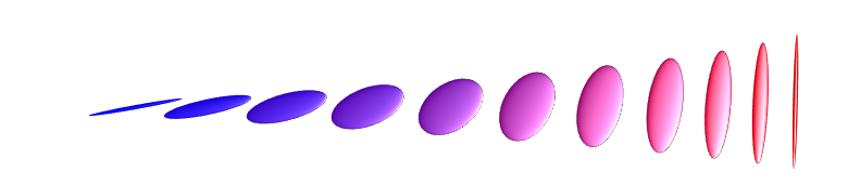
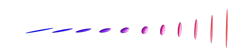
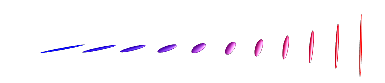
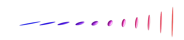
Interpolation of \(3 \times 3\) SPD matrices between two anisotropic tensors with different principal directions, reproduced from Lin (2019). Top: Euclidean linear interpolation shows a pronounced swelling effect — the interpolated ellipsoids become artificially rounder and more isotropic, with determinants ballooning from 5.40 to over 40. Remaining rows: Affine-invariant, Log-Euclidean, and Log-Cholesky geodesic interpolations all preserve the shape characteristics and exhibit smooth, monotonic determinant evolution, confirming they are free of the swelling artifact.
6.2 Intrinsic Geometries
A widely used intrinsic geometry is given by the affine-invariant distance:
\[ d_{\mathrm{AI}}(\Sigma_0, \Sigma_1) = \bigl\|\log(\Sigma_0^{-1/2}\Sigma_1\Sigma_0^{-1/2})\bigr\|_F, \]
where \(\|\cdot\|_F\) denotes the Frobenius norm and \(\log\) denotes the principal matrix logarithm. The associated Riemannian metric is
\[ g_{\Sigma}(U, V) = \operatorname{tr}\bigl(\Sigma^{-1}U\,\Sigma^{-1}V\bigr), \]
under which \(\mathcal{S}_{++}^{m}\) is a Hadamard manifold whose sectional curvatures lie between \(-1/2\) and \(0\) (Pennec et al. 2006; Thanwerdas and Pennec 2023).
An alternative is the log-Euclidean distance (Arsigny et al. 2006, 2007):
\[ d_{\mathrm{LE}}(\Sigma_0, \Sigma_1) = \|\log \Sigma_0 - \log \Sigma_1\|_F. \]
Equivalently, in the log-Euclidean framework, one maps SPD matrices by the matrix logarithm into the linear space of symmetric matrices, performs Euclidean calculations there, and maps back by the matrix exponential. Another recent alternative is the log-Cholesky metric, which is built from the Cholesky decomposition and yields a computationally convenient Riemannian geometry on SPD matrices (Lin 2019).
The intrinsic geometries described below rely on the matrix exponential \(\exp(\cdot)\) and the principal matrix logarithm \(\log(\cdot)\), which map between the space of symmetric matrices and the space of SPD matrices.
Spectral decomposition. Every SPD matrix \(\Sigma \in \mathcal{S}_{++}^{m}\) admits a spectral decomposition
\[ \Sigma = U \Lambda U^\top = \sum_{i=1}^{m} \lambda_i\, u_i u_i^\top, \]
where \(U\) is orthogonal (\(U^\top U = I_m\)) and \(\Lambda = \operatorname{diag}(\lambda_1, \ldots, \lambda_m)\) with strictly positive eigenvalues \(\lambda_i > 0\).
Matrix logarithm. The principal matrix logarithm applies \(\log\) to each eigenvalue:
\[ \log(\Sigma) = U \operatorname{diag}\bigl(\log \lambda_1, \ldots, \log \lambda_m\bigr) U^\top. \]
Since \(\lambda_i > 0\), \(\log \lambda_i\) is well-defined and real. The result \(\log(\Sigma)\) is a symmetric matrix (no longer required to be positive definite). Thus \(\log : \mathcal{S}_{++}^{m} \to \mathcal{S}^{m}\), where \(\mathcal{S}^{m}\) is the vector space of \(m \times m\) symmetric matrices.
Matrix exponential. Conversely, for any symmetric matrix \(S = V \Phi V^\top \in \mathcal{S}^{m}\) (with arbitrary real eigenvalues \(\phi_i\)), the matrix exponential is
\[ \exp(S) = V \operatorname{diag}\bigl(e^{\phi_1}, \ldots, e^{\phi_m}\bigr) V^\top. \]
Because \(e^{\phi_i} > 0\) for all real \(\phi_i\), the result \(\exp(S)\) is always SPD. Thus \(\exp : \mathcal{S}^{m} \to \mathcal{S}_{++}^{m}\).
Key property. The maps \(\exp\) and \(\log\) are mutual inverses: \(\exp(\log(\Sigma)) = \Sigma\) for all \(\Sigma \in \mathcal{S}_{++}^{m}\), and \(\log(\exp(S)) = S\) for all \(S \in \mathcal{S}^{m}\). This bijection is the foundation of the Log-Euclidean framework, which transfers computations from the curved SPD manifold to the flat vector space of symmetric matrices via the matrix logarithm, and maps results back via the matrix exponential.
7 Example: Spherical and Compositional Data
Directional observations such as paleomagnetic directions, wind directions, and fiber orientations naturally live on spheres, while compositional observations such as geochemical percentages, microbiome relative abundances, and budget shares live on simplices (Fisher 1953; Kent 1982; Aitchison 1982; Egozcue et al. 2003).
The sphere is the manifold
\[ \mathbb{S}^{p-1} = \{x \in \mathbb{R}^p : \|x\|_2 = 1\}, \]
typically equipped with the geodesic distance
\[ d_{\mathbb{S}}(x, y) = \arccos\bigl(\langle x, y \rangle\bigr). \]


Compositional data with \(p\) parts take values in the open simplex
\[ \Delta^{p-1} = \Bigl\{x = (x_1, \ldots, x_p) \in (0, \infty)^p : \sum_{i=1}^p x_i = 1\Bigr\}. \]
After the reparameterization \((x_1, \ldots, x_p) \mapsto (\sqrt{x_1}, \ldots, \sqrt{x_p})\), we can view \(\Delta^{p-1}\) as a subspace of \(\mathbb{S}^{p-1}\).
The sphere is genuinely non-Euclidean: it is not closed under vector addition, has positive curvature, and geodesics are great-circle arcs rather than straight lines in the ambient space.
8 Example: Distributional Data (Wasserstein Space)
In many modern problems, each observation is itself a probability distribution — for example, an age-at-death distribution, an income distribution, or an intensity distribution extracted from imaging data. For distributions on \(\mathbb{R}^p\), the most common choice is
\[ \mathcal{P}_2(\mathbb{R}^p) = \Bigl\{\mu : \mu \text{ is a Borel probability measure on } \mathbb{R}^p \text{ and } \int_{\mathbb{R}^p} \|x\|_2^2\,d\mu(x) < \infty\Bigr\}, \]
equipped with the quadratic Wasserstein distance
\[ W_2^2(\mu, \nu) = \inf_{\pi \in \Pi(\mu, \nu)} \int_{\mathbb{R}^p \times \mathbb{R}^p} \|x-y\|_2^2\,d\pi(x, y), \]
where \(\Pi(\mu, \nu)\) denotes the set of all couplings with marginals \(\mu\) and \(\nu\).
Wasserstein space is not Euclidean in general because:
- Arbitrary linear combinations of probability measures may not yield probability measures.
- There is no global finite-dimensional linear structure compatible with the Wasserstein distance.
- In general, Wasserstein spaces are infinite-dimensional.
- For dimensions \(p \ge 2\), the geometry is genuinely curved.
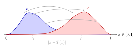
In one dimension, the map \(\mu \mapsto F^{-1}_{\mu}\) (the quantile function) identifies \((\mathcal{P}_2(\mathbb{R}), W_2)\) isometrically with a convex subset of \(L^2(0,1)\), which explains why one-dimensional Wasserstein statistics are often especially tractable.
9 Metric Spaces vs. Riemannian Manifolds
In the examples above, the SPD space and the sphere carry more structure — specifically, a Riemannian manifold structure. Below is a high-level comparison of the two viewpoints:
| General Metric Spaces | Riemannian Manifolds | |
|---|---|---|
| Structural input | Only a distance \(d\) | Charts, metric, exp/log maps, curvature |
| Scope | Very broad (incl. singular spaces) | Smooth spaces only |
| Computation | Often hard (no gradients) | Easier (gradient descent, linearization) |
| Theory | Indirect (metric entropy, comparison) | Direct (Taylor, Jacobi fields, connections) |
| Tradeoff | Easy to define, hard to analyze | Harder to set up, easier once in place |
On the one hand, the metric-space viewpoint is maximally flexible: once a meaningful distance is available, one can define Fréchet means, variances, regression functions, and other statistical targets. On the other hand, this generality comes at a price. Without tangent spaces, gradients, or local coordinates, both computation and theory often have to be built from indirect tools such as convexity along geodesics, comparison geometry, empirical-process bounds, and metric entropy.
By contrast, Riemannian manifolds demand substantially more geometric machinery at the outset, but once that machinery is available, many statistical problems become more tractable because one can differentiate, locally linearize, and optimize intrinsically.
Related terminology for non-Euclidean data varies. One sees object data in La Rosa et al. (2012); the broader phrase object-oriented data analysis in Wang and Marron (2007) and Marron and Alonso (2014); random objects in Petersen and Müller (2019); and manifold-valued data in Lin et al. (2017). In geometry-first applications, one also encounters broader descriptions in terms of geometric data or geometry-and-statistics on manifolds and stratified spaces (Feragen et al. 2014). These labels are not identical, but they refer to closely related situations in which the observations are complex objects rather than ordinary Euclidean vectors.
10 Roadmap of the Notes
The remaining lectures follow a general-to-structured progression. We begin with statistical methods that require only a metric, develop regression and classification for metric-space-valued data, study probability distributions through Wasserstein geometry, and finally exploit the differentiable structure of Riemannian manifolds.
10.1 Part I: Fréchet Means in General Metric Spaces
- Lecture 2: Existence and uniqueness. We define population and sample Fréchet means, examine why minimizers may fail to exist or be unique, and obtain existence and uniqueness from compactness, geodesic convexity, curvature bounds, and Hadamard-space geometry.
- Lecture 3: Consistency and convergence rates. We establish strong consistency, introduce covering and packing numbers and metric entropy, derive convergence rates for Fréchet means, and discuss nonclassical phenomena such as stickiness and smeariness.
- Lecture 4: Inference in general metric spaces. We develop inference without subtraction, tangent spaces, or covariance matrices, using the scalar Fréchet variance, multi-sample Fréchet ANOVA, isotropic randomization tests, and confidence sets.
- Lecture 5: Computation. We turn the Fréchet mean problem into an algorithmic one, introducing proximal maps and cyclic and randomized split proximal-point algorithms in Hadamard spaces.
10.2 Part II: Regression and Classification with Metric-Space Data
- Lecture 6: Global Fréchet regression. We extend linear regression to metric-space responses by expressing Euclidean regression as a weighted least-squares problem and replacing squared Euclidean loss with squared metric distance.
- Lecture 7: Kernel Fréchet regression. We construct a local-constant, Nadaraya–Watson-type estimator for nonlinear conditional Fréchet means and study bandwidth selection, computation, and the bias–variance tradeoff.
- Lecture 8: Local Fréchet regression. We use local-linear weights to reduce boundary bias and develop the bias, stochastic-error, convergence-rate, and bandwidth theory of local Fréchet regression.
- Lecture 9: Total-variation regularized Fréchet regression. For trajectories with abrupt changes, we replace smoothness by a metric total-variation penalty, leading to piecewise-constant fits, change-point detection, proximal computation, and minimax convergence rates.
- Lecture 10: Logistic regression with metric-space covariates. We reverse the roles of predictor and response: the outcome is binary and the predictor is a nonlinear object. An Alexandrov inner product, a Fréchet-mean anchor, and a coefficient object provide a geometry-respecting classifier.
10.3 Part III: Wasserstein Geometry and Distribution-Valued Data
- Lecture 11: Wasserstein distance and geometry. We introduce optimal couplings, optimal transport maps, displacement interpolation, the one-dimensional quantile representation, and the curvature properties of Wasserstein spaces.
- Lecture 12: Wasserstein barycenters. We specialize Fréchet means to probability measures, deriving explicit one-dimensional and Gaussian barycenters and studying their existence, consistency, rates, and computation.
- Lecture 13: Probability distributions from samples. We investigate empirical measures and plug-in Wasserstein distances, including consistency, distributional limits, intrinsic Wasserstein dimension, and the curse of dimensionality.
- Lecture 14: Distribution-on-distribution regression. We compare transformation-based and intrinsic regression for distributions, using Wasserstein log and exponential maps, tangent-space linearization, and optimal-transport-map regression.
10.4 Part IV: Riemannian Statistical Methods
- Lecture 15: Riemannian foundations. We introduce smooth manifolds, charts, tangent spaces, Riemannian metrics, geodesics, exponential and logarithmic maps, the cut locus, connections, and curvature, with the sphere and SPD cone as principal examples.
- Lecture 16: Fréchet means on manifolds. Differentiability yields the intrinsic first-order condition \(\mathbb{E}\{\log_\mu(X)\}=0\), sharper existence and uniqueness results, parametric convergence rates, and Riemannian gradient algorithms.
- Lecture 17: Central limit theorems for intrinsic means. We derive asymptotic normality in tangent coordinates, interpret the curvature-dependent sandwich covariance, address cut-locus and singular-Hessian complications, and construct confidence regions.
- Lecture 18: Geodesic regression. We model the conditional mean as a geodesic, estimate its intercept and tangent-space slope by intrinsic least squares, and assess fit through an intrinsic \(R^2\) and permutation testing.
- Lecture 19: Intrinsic local polynomial regression. We locally linearize manifold-valued responses in a tangent space, fit polynomial approximations, and compare these structure-aware estimators with metric-only local Fréchet regression.
This organization makes the tradeoff between generality and structure explicit. The early methods remain valid for arbitrary metric-space data; the Wasserstein lectures exploit the special geometry of probability measures; and the final lectures show what becomes possible when smooth manifold structure supplies tangent vectors, derivatives, and local linear approximations.
11 Key Takeaways
- Classical statistics implicitly depends on Euclidean structure — linear combinations, inner products, norms, straight-line interpolation.
- Many modern data objects cannot be represented as unconstrained vectors: trees, SPD matrices, directions, compositions, and probability distributions all violate Euclidean structure.
- Non-Euclidean ≠ exotic — these data types arise naturally in biology, medicine, geoscience, computer vision, and economics.
- A space can fail to be Euclidean at distinct structural levels, from lacking a metric entirely to being infinite-dimensional.
- These notes focus on metric spaces as the minimal structure for statistical analysis.
- Metric-space generality trades off against Riemannian tractability: we develop both and apply each where it is most useful.
12 Exercises
Parallelogram law: Prove that if \((\mathcal{M}, \|\cdot\|)\) is a normed space whose norm satisfies the parallelogram law, then \(\langle u, v \rangle := \tfrac{1}{4}(\|u+v\|^2 - \|u-v\|^2)\) defines an inner product that induces \(\|\cdot\|\). 📝 Show Solution
Non-Euclidean classification: For each of the following spaces, identify which of the five structural levels it fails at:
- The space of probability distributions on \(\{1, \ldots, K\}\) with total variation distance.
- The space of \(m \times m\) orthogonal matrices with the Frobenius distance.
- A finite graph with shortest-path distance. 📝 Show Solution
BHV tree space: For rooted binary \(3\)-trees, the BHV space consists of three rays glued at the origin. Sketch this space and compute \(d_{\mathrm{BHV}}(T_1, T_2)\) for two trees on different rays. 📝 Show Solution
Swelling effect: Let \(\Sigma_1 = \operatorname{diag}(a, 1/a)\) and \(\Sigma_2 = \operatorname{diag}(1/a, a)\) for \(a > 1\). Compute the Euclidean mean \(\tfrac{1}{2}(\Sigma_1 + \Sigma_2)\) and compare its determinant to those of \(\Sigma_1\) and \(\Sigma_2\). Verify the swelling effect. 📝 Show Solution
Arc length distance on the sphere: Show that the arc length (geodesic) distance \(d(x,y) = \arccos(\langle x, y \rangle)\) defines a metric on the sphere \(\mathbb{S}^{p-1}\). That is, verify that it satisfies positivity, symmetry, and the triangle inequality. 📝 Show Solution
13 Further Reading
- Billera et al. (2001) — The original BHV tree space construction.
- Pennec et al. (2006) — Riemannian geometry for SPD matrices with medical imaging applications.
- Burago et al. (2001) — A comprehensive introduction to metric geometry, covering length spaces, Alexandrov curvature, and the geometry of metric spaces.
- Lee (2018) — A clear, modern introduction to Riemannian manifolds covering metrics, connections, geodesics, and curvature.
14 Self-Assessment Quiz
Test your understanding of this lecture with the interactive MCQ quiz: