---
title: "Lecture 15: Riemannian Manifolds — Foundations"
subtitle: "Smooth manifolds, tangent spaces, metrics, and curvature"
format:
html:
code-fold: true
code-tools: true
code-copy: true
pdf:
documentclass: scrartcl
pdf-engine: xelatex
toc: true
number-sections: true
geometry:
- margin=1in
colorlinks: true
bibliography: source/ref.bib
---
## Learning Goals
By the end of this lecture, learners should be able to:
- Define topological and smooth manifolds, charts, atlases, and transition maps, and visualize them on $\mathbb{S}^2$ using stereographic charts.
- Visualize the tangent space $T_p\mathcal{M}$ as a vector space attached to a point, with a coordinate-derived tangent frame.
- State the definitions of Riemannian metric, geodesic, exponential map, and logarithmic map.
- Explain the inverse relationship $\exp_p(\log_p(q)) = q$ and why it fails at the cut locus.
- Compute the gradient of the squared-distance function on a Riemannian manifold.
- Explain the Levi-Civita connection and the meaning of sectional curvature.
- Contrast Hadamard manifolds with positively curved manifolds.
- Describe the SPD cone and the sphere as Riemannian manifolds with explicit metrics.
## Topological and Smooth Manifolds
::: {#def-topological-manifold .definition title="Topological manifold"}
A topological space $\mathcal{M}$ is a **topological manifold of dimension $m$** if it is Hausdorff, second countable, and every point $p \in \mathcal{M}$ has an open neighborhood $U$ homeomorphic to an open subset of $\mathbb{R}^m$.
:::
::: {.callout-note appearance="simple" collapse="true" title="A Quick Primer on Topology"}
**Topology** is the study of properties of spaces that are preserved under continuous deformations — stretching, bending, twisting — but not tearing or gluing. A **topological space** $(X, \tau)$ is a set $X$ together with a collection $\tau$ of subsets (called *open sets*) satisfying three axioms: (i) $\emptyset$ and $X$ are open, (ii) arbitrary unions of open sets are open, and (iii) finite intersections of open sets are open. The open sets define a notion of "nearness" without needing a distance function.
Three key properties appear in the definition of a topological manifold:
**Hausdorff ($T_2$).** Any two distinct points can be separated by disjoint open neighborhoods. This rules out pathological spaces where sequences can converge to two different limits at once.
- *Example:* $\mathbb{R}^n$ with the usual Euclidean topology is Hausdorff — two distinct points $x \neq y$ can be enclosed in disjoint open balls of radius $\|x-y\|/3$.
**Second countable.** There exists a countable basis for the topology — a countable collection $\mathcal{B}$ of open sets such that every open set can be written as a union of members of $\mathcal{B}$. This ensures the manifold is "not too big" and guarantees existence of partitions of unity (a crucial tool for constructing Riemannian metrics).
- *Example:* $\mathbb{R}^n$ is second countable — take $\mathcal{B}$ as all open balls with rational centers and rational radii. There are only countably many such balls, and any open set is a union of them.
**Homeomorphism.** A continuous bijection with a continuous inverse. Two spaces are homeomorphic if one can be continuously deformed into the other without cutting or gluing.
- *Example:* A coffee cup and a donut (torus) are homeomorphic — stretch the handle, deform the cup body, and they match.
- *Example:* A sphere $\mathbb{S}^2$ is **not** homeomorphic to a torus $\mathbb{T}^2$ — you cannot remove the hole without tearing (they have different genus).
:::
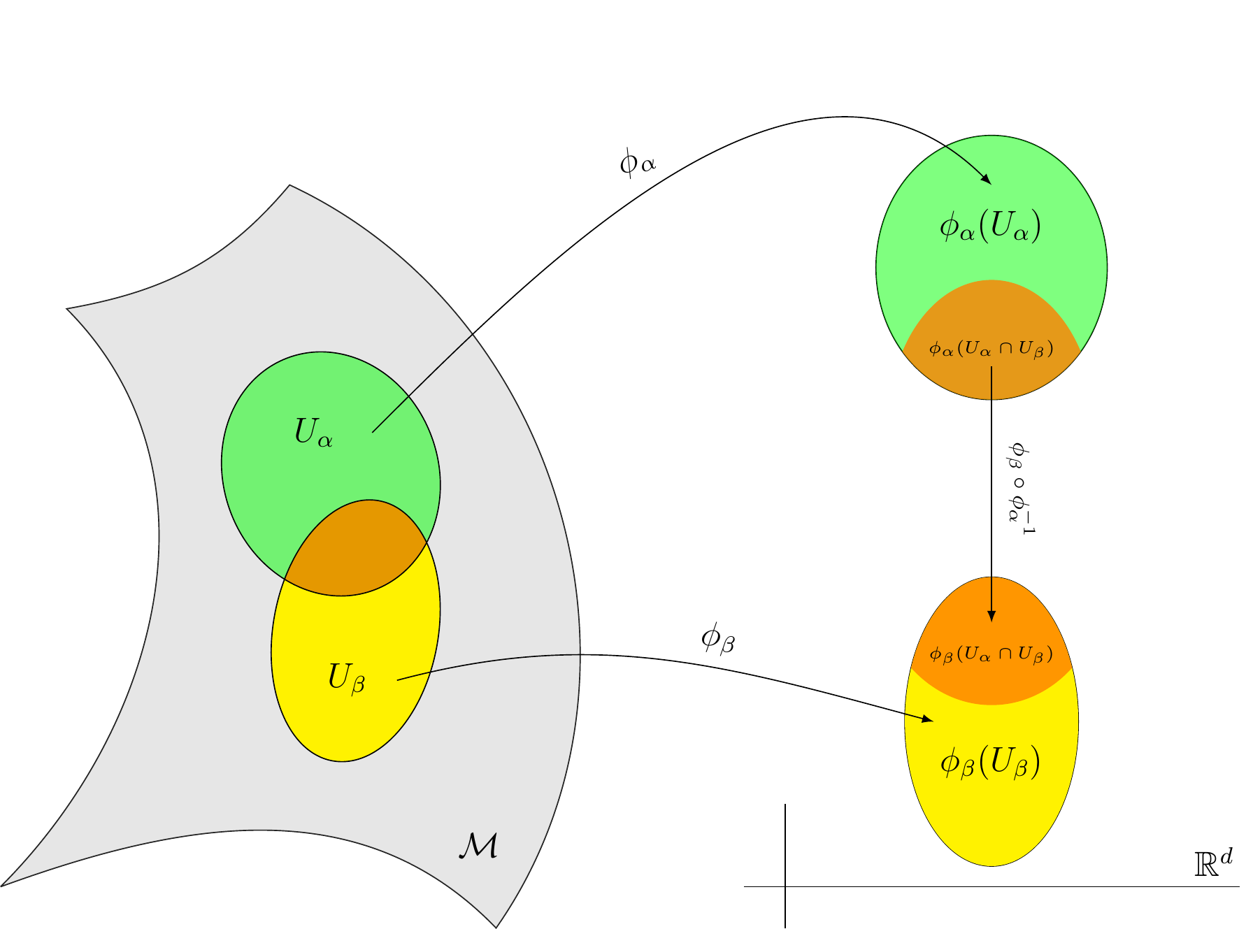
If $U \subset \mathcal{M}$ is open and $\phi : U \to \phi(U) \subset \mathbb{R}^m$ is such a homeomorphism, then $(U, \phi)$ is called a **chart**. A collection of charts covering $\mathcal{M}$ is an **atlas**. On overlaps $(U_\alpha, \phi_\alpha)$ and $(U_\beta, \phi_\beta)$, the **transition map** $\phi_\alpha \circ \phi_\beta^{-1}$ relates the two coordinate systems.
{width=80%}
::: {#def-smooth-manifold .definition title="Smooth manifold"}
For $k \ge 1$, a $C^k$-atlas has $k$-times continuously differentiable transition maps. A **smooth manifold** is a topological manifold with a maximal compatible $C^\infty$-atlas.
:::
::: {.callout-note appearance="simple" collapse="true" title="What does "maximal compatible" mean?"}
Two $C^\infty$-atlases are **compatible** if their union is still a $C^\infty$-atlas — equivalently, every chart from one atlas has smooth transition maps with every chart from the other. Compatibility is an equivalence relation on atlases; a **smooth structure** on $\mathcal{M}$ is an equivalence class under this relation.
A **maximal atlas** is the union of *all* charts belonging to *any* atlas in a given equivalence class. It is the unique largest atlas in that class — throw in every compatible chart and you get the maximal one.
**Why bother?** Defining a smooth manifold as "a topological manifold *together with a maximal* $C^\infty$-atlas" makes the smooth structure unambiguous without privileging a particular set of charts. In practice, you only need to exhibit *one* $C^\infty$-atlas on $\mathcal{M}$; it uniquely determines the maximal atlas, so the smooth structure is well-defined.
**Example.** The stereographic atlas on $\mathbb{S}^2$ (the two charts $(U_N, \phi_N)$ and $(U_S, \phi_S)$ defined below) is not maximal — you could add, say, a rotated version of the north-pole chart. But the stereographic atlas already determines the smooth structure: the maximal atlas is simply every chart on $\mathbb{S}^2$ whose transition maps with both stereographic charts are $C^\infty$.
:::
### Examples
**Example 1: The 2-sphere $\mathbb{S}^2$.** The unit sphere $\mathbb{S}^2 = \{x \in \mathbb{R}^3 : \|x\|_2 = 1\}$ is a 2-dimensional smooth manifold. It cannot be covered by a single chart (it is compact, whereas a nonempty open subset of $\mathbb{R}^2$ is not), and the following two stereographic charts form a minimal atlas.
::: {.example title="Stereographic atlas of $\mathbb{S}^2$"}
**North-pole chart $(U_N, \phi_N)$.** Let $N = (0, 0, 1)$ be the north pole. Define $U_N = \mathbb{S}^2 \setminus \{N\}$ and $\phi_N : U_N \to \mathbb{R}^2$ by
$$
\phi_N(x_1, x_2, x_3) = \left(\frac{x_1}{1 - x_3},\; \frac{x_2}{1 - x_3}\right).
$$
Geometrically, $\phi_N$ projects from $N$ onto the equatorial plane $\{x_3 = 0\}$. The inverse is
$$
\phi_N^{-1}(u, v) = \left(\frac{2u}{1 + u^2 + v^2},\; \frac{2v}{1 + u^2 + v^2},\; \frac{u^2 + v^2 - 1}{1 + u^2 + v^2}\right).
$$
**South-pole chart $(U_S, \phi_S)$.** Let $S = (0, 0, -1)$ be the south pole. Define $U_S = \mathbb{S}^2 \setminus \{S\}$ and $\phi_S : U_S \to \mathbb{R}^2$ by
$$
\phi_S(x_1, x_2, x_3) = \left(\frac{x_1}{1 + x_3},\; \frac{x_2}{1 + x_3}\right).
$$
**Transition map.** On the overlap $U_N \cap U_S = \mathbb{S}^2 \setminus \{N, S\}$, both charts are defined. The transition map $\phi_S \circ \phi_N^{-1} : \mathbb{R}^2 \setminus \{(0,0)\} \to \mathbb{R}^2 \setminus \{(0,0)\}$ is
$$
(\phi_S \circ \phi_N^{-1})(u, v) = \left(\frac{u}{u^2 + v^2},\; \frac{v}{u^2 + v^2}\right).
$$
This is $C^\infty$ on $\mathbb{R}^2 \setminus \{(0,0)\}$, confirming that $\{(U_N, \phi_N), (U_S, \phi_S)\}$ is a smooth atlas. The point $(0,0)$ is not in the overlap because $\phi_N^{-1}(0,0) = S$ and $\phi_S^{-1}(0,0) = N$ — each pole is covered by exactly one chart.
:::
**Example 2: The SPD cone $\mathcal{S}_{++}^m$.** Let $\operatorname{Sym}(m) = \{A \in \mathbb{R}^{m \times m} : A^\top = A\}$ be the vector space of symmetric matrices, of dimension $m(m+1)/2$. The set
$$
\mathcal{S}_{++}^m = \{\Sigma \in \operatorname{Sym}(m) : x^\top \Sigma x > 0 \text{ for all } x \in \mathbb{R}^m \setminus \{0\}\}
$$
is an **open subset** of $\operatorname{Sym}(m)$ (the cone of positive-definite matrices). Being an open subset of a finite-dimensional vector space, $\mathcal{S}_{++}^m$ is a smooth manifold of dimension $m(m+1)/2$.
::: {.example title="Global chart for $\mathcal{S}_{++}^m$ via the matrix logarithm"}
Since $\mathcal{S}_{++}^m$ is an open subset of a vector space, a **single chart** (a global atlas) suffices. The most natural chart is the identity inclusion; a more useful one in practice is the **matrix logarithm** chart.
Let $\operatorname{vech} : \operatorname{Sym}(m) \to \mathbb{R}^{m(m+1)/2}$ be the half-vectorization operator that stacks the $m(m+1)/2$ unique entries of a symmetric matrix into a vector (e.g., column-wise, excluding the strict upper triangle). Define the global chart
$$
\phi : \mathcal{S}_{++}^m \to \mathbb{R}^{m(m+1)/2}, \qquad \phi(\Sigma) = \operatorname{vech}(\log \Sigma),
$$
where $\log$ is the principal matrix logarithm. This is a homeomorphism because $\log : \mathcal{S}_{++}^m \to \operatorname{Sym}(m)$ is a diffeomorphism with smooth inverse $\exp : \operatorname{Sym}(m) \to \mathcal{S}_{++}^m$ (the matrix exponential). The chart domain is all of $\mathcal{S}_{++}^m$, so $\{(\mathcal{S}_{++}^m, \phi)\}$ is a one-chart smooth atlas.
**For $m = 2$ (used in the portfolio demos in Lectures 6–10),** $\operatorname{Sym}(2)$ has dimension $3$. Writing $\Sigma = \begin{pmatrix} a & b \\ b & c \end{pmatrix}$,
$$
\phi(\Sigma) = \operatorname{vech}(\log \Sigma) = \begin{pmatrix} [\log \Sigma]_{11} \\ [\log \Sigma]_{12} \\ [\log \Sigma]_{22} \end{pmatrix} \in \mathbb{R}^3.
$$
This is the coordinate representation used throughout the interactive demos in earlier lectures, where the compact storage `[a, b, c]` represents the three independent entries of the log-covariance matrix.
:::
**Other examples:** Grassmann manifolds $\mathrm{Gr}(r,m)$ (subspaces), $\mathrm{SO}(m)$ (rotations), hyperbolic spaces (hierarchical data), Kendall shape spaces (landmark configurations).
### Interactive: Charts, Atlas, and Transition Maps on $\mathbb{S}^2$
The abstract definition of charts and atlases becomes concrete when visualized on the sphere. The following demo shows two stereographic charts — one from the north pole, one from the south pole — that together form an atlas for $\mathbb{S}^2$. Pick a point on the sphere to see its coordinates in each chart and the transition map between them.
```{ojs}
//| label: fig-chart-atlas
//| fig-cap: "Interactive: Charts, atlas, and transition maps on the 2-sphere"
chart_th_control = Inputs.range([0, 180], {step: 1, value: 45, label: "Point θ (colatitude °)"})
chart_ph_control = Inputs.range([0, 360], {step: 5, value: 120, label: "Point φ (longitude °)"})
chart_rotY_control = Inputs.range([0, 360], {step: 10, value: 200, label: "Chart view azimuth °"})
chart_rotX_control = Inputs.range([-50, 50], {step: 5, value: 20, label: "Chart view elevation °"})
chart_th = Generators.input(chart_th_control)
chart_ph = Generators.input(chart_ph_control)
chart_rotY = Generators.input(chart_rotY_control)
chart_rotX = Generators.input(chart_rotX_control)

chart_controls_view = html`
<style>
  .chart-slider-grid { display:grid; grid-template-columns:repeat(2,minmax(0,1fr)); gap:6px 20px; max-width:700px; margin:0 auto 12px; font:0.85em system-ui,sans-serif; }
  .chart-slider-grid > * { min-width:0; margin:0; }
  .chart-slider-grid input[type="number"] { width:7.5rem !important; }
  .chart-atlas-layout { display:flex; gap:20px; flex-wrap:wrap; align-items:flex-start; }
  .chart-s2-wrap { flex:0 1 380px; min-width:0; }
  .chart-s2-globe { display:block; width:100%; max-width:380px; height:auto; }
  .chart-atlas-details { flex:1 1 360px; min-width:min(100%,330px); }
  .chart-plane-grid { display:grid; grid-template-columns:repeat(2,minmax(0,1fr)); gap:10px; margin-bottom:12px; }
  .chart-plane-card { min-width:0; padding:8px; border:1px solid #dee2e6; border-radius:6px; background:#fff; }
  .chart-plane-card h5 { margin:0 0 4px; text-align:center; font-size:0.85em; }
  .chart-plane-card svg { display:block; width:100%; height:auto; }
  @media (max-width:500px) { .chart-slider-grid { grid-template-columns:1fr; } }
  @media (max-width:500px) { .chart-plane-grid { grid-template-columns:1fr; } }
</style>
<div class="chart-slider-grid">
  <div>${chart_th_control}</div>
  <div>${chart_ph_control}</div>
  <div>${chart_rotY_control}</div>
  <div>${chart_rotX_control}</div>
</div>`

function attachS2DragRotation(root, selector, azimuthLabel, elevationLabel, minElevation, maxElevation, data, kind) {
  var svg = root.querySelector(selector);
  if (!svg) return root;
  var scene = svg.querySelector('g[transform^="translate"]');
  if (!scene) return root;

  function findRange(labelText) {
    var labels = Array.from(document.querySelectorAll("label"));
    for (var i = 0; i < labels.length; i++) {
      if (labels[i].textContent.indexOf(labelText) >= 0) {
        return labels[i].querySelector('input[type="range"]') ||
          (labels[i].parentElement && labels[i].parentElement.querySelector('input[type="range"]'));
      }
    }
    return null;
  }

  var az = findRange(azimuthLabel);
  var el = findRange(elevationLabel);
  var state = {
    rotY: az ? Number(az.value) : 200,
    rotX: el ? Number(el.value) : 20
  };

  function clamp(x, lo, hi) {
    return Math.max(lo, Math.min(hi, x));
  }

  function makeProjector(rotY, rotX, R) {
    var ry = rotY * Math.PI / 180;
    var rx = rotX * Math.PI / 180;
    return function(v) {
      var x1 = v[0]*Math.cos(ry) + v[2]*Math.sin(ry);
      var y1 = v[1];
      var z1 = -v[0]*Math.sin(ry) + v[2]*Math.cos(ry);
      var x2 = x1;
      var y2 = y1*Math.cos(rx) - z1*Math.sin(rx);
      var z2 = y1*Math.sin(rx) + z1*Math.cos(rx);
      return {x: x2*R, y: -y2*R, z: z2};
    };
  }

  function renderWireframe(parts, proj, R, opacity) {
    for (var p = 0; p <= 18; p++) {
      var z = 1 - p*2/18;
      var r = Math.sqrt(Math.max(0, 1 - z*z));
      var d = '';
      for (var j = 0; j <= 120; j++) {
        var phi = j*2*Math.PI/120;
        var pt = proj([r*Math.cos(phi), r*Math.sin(phi), z]);
        d += (j===0?'M':'L')+' '+pt.x.toFixed(1)+' '+pt.y.toFixed(1);
      }
      parts.push('<path d="'+d+'" fill="none" stroke="#adb5bd" stroke-width="0.5" opacity="'+opacity+'"/>');
    }
    for (var m = 0; m < 24; m++) {
      var mphi = m*Math.PI/12;
      var md = '';
      for (var mj = 0; mj <= 90; mj++) {
        var theta = mj*Math.PI/90;
        var mpt = proj([Math.sin(theta)*Math.cos(mphi), Math.sin(theta)*Math.sin(mphi), Math.cos(theta)]);
        md += (mj===0?'M':'L')+' '+mpt.x.toFixed(1)+' '+mpt.y.toFixed(1);
      }
      parts.push('<path d="'+md+'" fill="none" stroke="#adb5bd" stroke-width="0.5" opacity="'+opacity+'"/>');
    }
    parts.push('<circle cx="0" cy="0" r="'+R+'" fill="none" stroke="#dee2e6" stroke-width="1.2"/>');
  }

  function renderChart(res, rotY, rotX) {
    var R = 160, parts = [];
    var proj = makeProjector(rotY, rotX, R);
    renderWireframe(parts, proj, R, 0.15);

    var nP = proj([0,0,1]);
    parts.push('<circle cx="'+nP.x.toFixed(1)+'" cy="'+nP.y.toFixed(1)+'" r="5" fill="#e03131"/>');
    parts.push('<line x1="'+(nP.x-4).toFixed(1)+'" y1="'+(nP.y-4).toFixed(1)+'" x2="'+(nP.x+4).toFixed(1)+'" y2="'+(nP.y+4).toFixed(1)+'" stroke="#fff" stroke-width="1.5"/>');
    parts.push('<line x1="'+(nP.x+4).toFixed(1)+'" y1="'+(nP.y-4).toFixed(1)+'" x2="'+(nP.x-4).toFixed(1)+'" y2="'+(nP.y+4).toFixed(1)+'" stroke="#fff" stroke-width="1.5"/>');
    parts.push('<text x="'+(nP.x+8).toFixed(0)+'" y="'+(nP.y-4).toFixed(0)+'" font-size="11" fill="#e03131" font-weight="bold">N</text>');
    var sP = proj([0,0,-1]);
    parts.push('<circle cx="'+sP.x.toFixed(1)+'" cy="'+sP.y.toFixed(1)+'" r="5" fill="#1971c2"/>');
    parts.push('<line x1="'+(sP.x-4).toFixed(1)+'" y1="'+(sP.y-4).toFixed(1)+'" x2="'+(sP.x+4).toFixed(1)+'" y2="'+(sP.y+4).toFixed(1)+'" stroke="#fff" stroke-width="1.5"/>');
    parts.push('<line x1="'+(sP.x+4).toFixed(1)+'" y1="'+(sP.y-4).toFixed(1)+'" x2="'+(sP.x-4).toFixed(1)+'" y2="'+(sP.y+4).toFixed(1)+'" stroke="#fff" stroke-width="1.5"/>');
    parts.push('<text x="'+(sP.x+8).toFixed(0)+'" y="'+(sP.y-4).toFixed(0)+'" font-size="11" fill="#1971c2" font-weight="bold">S</text>');
    var pP = proj(res.P);
    parts.push('<circle cx="'+pP.x.toFixed(1)+'" cy="'+pP.y.toFixed(1)+'" r="6" fill="#2b8a3e" stroke="#fff" stroke-width="2"/>');
    parts.push('<text x="'+(pP.x+10).toFixed(0)+'" y="'+(pP.y-6).toFixed(0)+'" font-size="11" fill="#2b8a3e" font-weight="bold">P</text>');
    return parts.join('\n');
  }

  function renderTangent(res, rotY, rotX) {
    var R = 175, parts = [];
    var proj = makeProjector(rotY, rotX, R);
    renderWireframe(parts, proj, R, 0.12);

    for (var i = 0; i < res.nGrid; i++) {
      var dRow = '';
      for (var j = 0; j < res.nGrid; j++) {
        var pt = proj(res.tgGrid[i*res.nGrid+j]);
        dRow += (j===0?'M':'L')+' '+pt.x.toFixed(1)+' '+pt.y.toFixed(1);
      }
      parts.push('<path d="'+dRow+'" fill="none" stroke="#f08c00" stroke-width="0.4" opacity="0.18"/>');
    }
    for (var cj = 0; cj < res.nGrid; cj++) {
      var dCol = '';
      for (var ci = 0; ci < res.nGrid; ci++) {
        var cpt = proj(res.tgGrid[ci*res.nGrid+cj]);
        dCol += (ci===0?'M':'L')+' '+cpt.x.toFixed(1)+' '+cpt.y.toFixed(1);
      }
      parts.push('<path d="'+dCol+'" fill="none" stroke="#f08c00" stroke-width="0.4" opacity="0.18"/>');
    }

    var cornerPts = [proj(res.tgGrid[0]), proj(res.tgGrid[res.nGrid-1]), proj(res.tgGrid[res.nGrid*res.nGrid-1]), proj(res.tgGrid[res.nGrid*(res.nGrid-1)])];
    var cStr = '';
    for (var ci2 = 0; ci2 < 4; ci2++) cStr += (ci2===0?'M':'L')+' '+cornerPts[ci2].x.toFixed(1)+' '+cornerPts[ci2].y.toFixed(1);
    parts.push('<path d="'+cStr+' Z" fill="none" stroke="#f08c00" stroke-width="1" opacity="0.3" stroke-dasharray="6,3"/>');

    var pP = proj(res.P);
    var etP = proj([res.P[0]+0.35*res.eTheta[0], res.P[1]+0.35*res.eTheta[1], res.P[2]+0.35*res.eTheta[2]]);
    var epP = proj([res.P[0]+0.35*res.ePhi[0], res.P[1]+0.35*res.ePhi[1], res.P[2]+0.35*res.ePhi[2]]);
    parts.push('<line x1="'+pP.x.toFixed(1)+'" y1="'+pP.y.toFixed(1)+'" x2="'+etP.x.toFixed(1)+'" y2="'+etP.y.toFixed(1)+'" stroke="#e03131" stroke-width="2"/>');
    parts.push('<text x="'+(etP.x+3).toFixed(0)+'" y="'+(etP.y-3).toFixed(0)+'" font-size="10" fill="#e03131">eθ</text>');
    parts.push('<line x1="'+pP.x.toFixed(1)+'" y1="'+pP.y.toFixed(1)+'" x2="'+epP.x.toFixed(1)+'" y2="'+epP.y.toFixed(1)+'" stroke="#1971c2" stroke-width="2"/>');
    parts.push('<text x="'+(epP.x+3).toFixed(0)+'" y="'+(epP.y-3).toFixed(0)+'" font-size="10" fill="#1971c2">eφ</text>');

    var vEnd = [res.P[0]+0.5*res.V[0], res.P[1]+0.5*res.V[1], res.P[2]+0.5*res.V[2]];
    var vdP = proj(vEnd);
    parts.push('<line x1="'+pP.x.toFixed(1)+'" y1="'+pP.y.toFixed(1)+'" x2="'+vdP.x.toFixed(1)+'" y2="'+vdP.y.toFixed(1)+'" stroke="#2b8a3e" stroke-width="3" stroke-linecap="round"/>');
    if (res.Vnorm > 0.01) {
      var vDir = [res.V[0]/res.Vnorm, res.V[1]/res.Vnorm, res.V[2]/res.Vnorm];
      var ahBase = [res.P[0]+0.42*res.V[0], res.P[1]+0.42*res.V[1], res.P[2]+0.42*res.V[2]];
      var orth = [vDir[1]*res.P[2]-vDir[2]*res.P[1], vDir[2]*res.P[0]-vDir[0]*res.P[2], vDir[0]*res.P[1]-vDir[1]*res.P[0]];
      var orthN = Math.sqrt(orth[0]*orth[0]+orth[1]*orth[1]+orth[2]*orth[2]);
      if (orthN > 1e-10) {
        orth = [orth[0]/orthN*0.08, orth[1]/orthN*0.08, orth[2]/orthN*0.08];
        var wing1 = [ahBase[0]+orth[0]-vDir[0]*0.06, ahBase[1]+orth[1]-vDir[1]*0.06, ahBase[2]+orth[2]-vDir[2]*0.06];
        var wing2 = [ahBase[0]-orth[0]-vDir[0]*0.06, ahBase[1]-orth[1]-vDir[1]*0.06, ahBase[2]-orth[2]-vDir[2]*0.06];
        var w1 = proj(wing1), w2 = proj(wing2);
        parts.push('<polygon points="'+vdP.x.toFixed(1)+','+vdP.y.toFixed(1)+' '+w1.x.toFixed(1)+','+w1.y.toFixed(1)+' '+w2.x.toFixed(1)+','+w2.y.toFixed(1)+'" fill="#2b8a3e"/>');
      }
    }
    parts.push('<text x="'+(vdP.x+5).toFixed(0)+'" y="'+(vdP.y-6).toFixed(0)+'" font-size="11" fill="#2b8a3e" font-weight="bold">v</text>');

    var geoPath = '';
    for (var gi = 0; gi < res.geodPts.length; gi++) {
      var gpt = proj(res.geodPts[gi]);
      geoPath += (gi===0?'M':'L')+' '+gpt.x.toFixed(1)+' '+gpt.y.toFixed(1);
    }
    parts.push('<path d="'+geoPath+'" fill="none" stroke="#7950f2" stroke-width="2.5" stroke-dasharray="8,4"/>');
    var expP = proj(res.expPt);
    parts.push('<circle cx="'+expP.x.toFixed(1)+'" cy="'+expP.y.toFixed(1)+'" r="5" fill="#7950f2" stroke="#fff" stroke-width="1.5"/>');
    parts.push('<text x="'+(expP.x+7).toFixed(0)+'" y="'+(expP.y-6).toFixed(0)+'" font-size="11" fill="#7950f2" font-weight="bold">expₚ(v)</text>');
    parts.push('<circle cx="'+pP.x.toFixed(1)+'" cy="'+pP.y.toFixed(1)+'" r="5.5" fill="#e03131" stroke="#fff" stroke-width="1.5"/>');
    parts.push('<text x="'+(pP.x+8).toFixed(0)+'" y="'+(pP.y-8).toFixed(0)+'" font-size="12" fill="#e03131" font-weight="bold">p</text>');
    return parts.join('\n');
  }

  function renderExpLog(res, rotY, rotX) {
    var R = 180, parts = [];
    var proj = makeProjector(rotY, rotX, R);
    renderWireframe(parts, proj, R, 0.12);

    for (var i = 0; i < res.nGrid; i++) {
      var dRow = '';
      for (var j = 0; j < res.nGrid; j++) {
        var pt = proj(res.tgGrid[i*res.nGrid+j]);
        dRow += (j===0?'M':'L')+' '+pt.x.toFixed(1)+' '+pt.y.toFixed(1);
      }
      parts.push('<path d="'+dRow+'" fill="none" stroke="#f08c00" stroke-width="0.3" opacity="0.15"/>');
    }
    for (var cj = 0; cj < res.nGrid; cj++) {
      var dCol = '';
      for (var ci = 0; ci < res.nGrid; ci++) {
        var cpt = proj(res.tgGrid[ci*res.nGrid+cj]);
        dCol += (ci===0?'M':'L')+' '+cpt.x.toFixed(1)+' '+cpt.y.toFixed(1);
      }
      parts.push('<path d="'+dCol+'" fill="none" stroke="#f08c00" stroke-width="0.3" opacity="0.15"/>');
    }

    function pathFrom(points) {
      var d = '';
      for (var i = 0; i < points.length; i++) {
        var pt = proj(points[i]);
        d += (i===0?'M':'L')+' '+pt.x.toFixed(1)+' '+pt.y.toFixed(1);
      }
      return d;
    }
    parts.push('<path d="'+pathFrom(res.geodExp)+'" fill="none" stroke="#7950f2" stroke-width="2.5" stroke-dasharray="8,4"/>');
    if (res.logDefined) parts.push('<path d="'+pathFrom(res.geodLog)+'" fill="none" stroke="#f08c00" stroke-width="2" stroke-dasharray="5,4"/>');

    var pP = proj(res.P);
    var vScale = 0.55/Math.max(1, res.Vnorm);
    var vdP = proj([res.P[0]+vScale*res.V[0], res.P[1]+vScale*res.V[1], res.P[2]+vScale*res.V[2]]);
    parts.push('<line x1="'+pP.x.toFixed(1)+'" y1="'+pP.y.toFixed(1)+'" x2="'+vdP.x.toFixed(1)+'" y2="'+vdP.y.toFixed(1)+'" stroke="#2b8a3e" stroke-width="3" stroke-linecap="round"/>');
    parts.push('<text x="'+(vdP.x+5).toFixed(0)+'" y="'+(vdP.y-7).toFixed(0)+'" font-size="11" fill="#2b8a3e" font-weight="bold">v</text>');
    if (res.logDefined) {
      var logScale = 0.55/Math.max(1, res.logNorm);
      var lqP = proj([res.P[0]+logScale*res.logQ[0], res.P[1]+logScale*res.logQ[1], res.P[2]+logScale*res.logQ[2]]);
      parts.push('<line x1="'+pP.x.toFixed(1)+'" y1="'+pP.y.toFixed(1)+'" x2="'+lqP.x.toFixed(1)+'" y2="'+lqP.y.toFixed(1)+'" stroke="#f08c00" stroke-width="2.5" stroke-linecap="round"/>');
      parts.push('<text x="'+(lqP.x+5).toFixed(0)+'" y="'+(lqP.y-7).toFixed(0)+'" font-size="11" fill="#f08c00" font-weight="bold">logₚ(q)</text>');
    }
    var expVP = proj(res.expV);
    parts.push('<circle cx="'+expVP.x.toFixed(1)+'" cy="'+expVP.y.toFixed(1)+'" r="5" fill="#7950f2" stroke="#fff" stroke-width="1.5"/>');
    parts.push('<text x="'+(expVP.x+6).toFixed(0)+'" y="'+(expVP.y-6).toFixed(0)+'" font-size="11" fill="#7950f2" font-weight="bold">expₚ(v)</text>');
    var qP = proj(res.Q);
    parts.push('<circle cx="'+qP.x.toFixed(1)+'" cy="'+qP.y.toFixed(1)+'" r="5" fill="#1971c2" stroke="#fff" stroke-width="1.5"/>');
    parts.push('<text x="'+(qP.x+6).toFixed(0)+'" y="'+(qP.y-6).toFixed(0)+'" font-size="11" fill="#1971c2" font-weight="bold">q</text>');
    parts.push('<circle cx="'+pP.x.toFixed(1)+'" cy="'+pP.y.toFixed(1)+'" r="5.5" fill="#e03131" stroke="#fff" stroke-width="1.5"/>');
    parts.push('<text x="'+(pP.x+8).toFixed(0)+'" y="'+(pP.y-8).toFixed(0)+'" font-size="12" fill="#e03131" font-weight="bold">p</text>');
    return parts.join('\n');
  }

  function renderPT(res, rotY, rotX) {
    var R = 175, parts = [];
    var proj = makeProjector(rotY, rotX, R);
    renderWireframe(parts, proj, R, 0.12);

    function pathFrom(points) {
      var d = '';
      for (var i = 0; i < points.length; i++) {
        var pt = proj(points[i]);
        d += (i===0?'M':'L')+' '+pt.x.toFixed(1)+' '+pt.y.toFixed(1);
      }
      return d;
    }

    parts.push('<path d="'+pathFrom(res.curve)+'" fill="none" stroke="#9775fa" stroke-width="1.1" stroke-dasharray="4,4" opacity="0.5"/>');
    if (res.trajPts.length > 1) {
      parts.push('<path d="'+pathFrom(res.trajPts)+'" fill="none" stroke="#7950f2" stroke-width="2.6"/>');
    }

    function drawArrow(base, vec, scl, color, w, op) {
      var tip = [base[0]+scl*vec[0], base[1]+scl*vec[1], base[2]+scl*vec[2]];
      var bP = proj(base), tP = proj(tip);
      var s = '<line x1="'+bP.x.toFixed(1)+'" y1="'+bP.y.toFixed(1)+'" x2="'+tP.x.toFixed(1)+'" y2="'+tP.y.toFixed(1)+'" stroke="'+color+'" stroke-width="'+w+'" stroke-linecap="round" opacity="'+op+'"/>';
      var vn = Math.sqrt(vec[0]*vec[0]+vec[1]*vec[1]+vec[2]*vec[2]);
      if (vn > 1e-9) {
        var vd = [vec[0]/vn, vec[1]/vn, vec[2]/vn];
        var ox = vd[1]*base[2]-vd[2]*base[1], oy = vd[2]*base[0]-vd[0]*base[2], oz = vd[0]*base[1]-vd[1]*base[0];
        var on = Math.sqrt(ox*ox+oy*oy+oz*oz);
        if (on > 1e-9) {
          ox /= on; oy /= on; oz /= on;
          var hl = Math.min(0.3*vn, 0.15), hw = Math.min(0.18*vn, 0.08);
          var wb = [tip[0]-scl*hl*vd[0], tip[1]-scl*hl*vd[1], tip[2]-scl*hl*vd[2]];
          var w1 = proj([wb[0]+scl*hw*ox, wb[1]+scl*hw*oy, wb[2]+scl*hw*oz]);
          var w2 = proj([wb[0]-scl*hw*ox, wb[1]-scl*hw*oy, wb[2]-scl*hw*oz]);
          s += '<polygon points="'+tP.x.toFixed(1)+','+tP.y.toFixed(1)+' '+w1.x.toFixed(1)+','+w1.y.toFixed(1)+' '+w2.x.toFixed(1)+','+w2.y.toFixed(1)+'" fill="'+color+'" opacity="'+op+'"/>';
        }
      }
      return s;
    }

    for (var ai = 0; ai < res.arrowSamples.length; ai++) {
      parts.push(drawArrow(res.arrowSamples[ai].p, res.arrowSamples[ai].v, 0.45, '#0ca678', 1.6, 0.85));
    }
    parts.push(drawArrow(res.P0, res.V0, 0.45, '#2b8a3e', 2, 0.4));
    parts.push(drawArrow(res.curPt, res.curVec, 0.45, '#2b8a3e', 3, 1));

    var tipV = proj([res.curPt[0]+0.45*res.curVec[0], res.curPt[1]+0.45*res.curVec[1], res.curPt[2]+0.45*res.curVec[2]]);
    parts.push('<text x="'+(tipV.x+5).toFixed(0)+'" y="'+(tipV.y-6).toFixed(0)+'" font-size="11" fill="#2b8a3e" font-weight="bold">V(t)</text>');

    var p0P = proj(res.P0);
    parts.push('<circle cx="'+p0P.x.toFixed(1)+'" cy="'+p0P.y.toFixed(1)+'" r="5.5" fill="#e03131" stroke="#fff" stroke-width="1.5"/>');
    parts.push('<text x="'+(p0P.x+8).toFixed(0)+'" y="'+(p0P.y-7).toFixed(0)+'" font-size="12" fill="#e03131" font-weight="bold">γ(0)</text>');
    var pcP = proj(res.curPt);
    parts.push('<circle cx="'+pcP.x.toFixed(1)+'" cy="'+pcP.y.toFixed(1)+'" r="5" fill="#7950f2" stroke="#fff" stroke-width="1.5"/>');
    parts.push('<text x="'+(pcP.x+7).toFixed(0)+'" y="'+(pcP.y-6).toFixed(0)+'" font-size="11" fill="#7950f2" font-weight="bold">γ(t)</text>');
    return parts.join('\n');
  }

  function render() {
    if (kind === "chart") scene.innerHTML = renderChart(data, state.rotY, state.rotX);
    if (kind === "tangent") scene.innerHTML = renderTangent(data, state.rotY, state.rotX);
    if (kind === "explog") scene.innerHTML = renderExpLog(data, state.rotY, state.rotX);
    if (kind === "pt") scene.innerHTML = renderPT(data, state.rotY, state.rotX);
  }

  var dragging = false;
  var lastX = 0;
  var lastY = 0;

  svg.addEventListener("pointerdown", function(event) {
    dragging = true;
    lastX = event.clientX;
    lastY = event.clientY;
    svg.setPointerCapture(event.pointerId);
    svg.style.cursor = "grabbing";
  });

  svg.addEventListener("pointermove", function(event) {
    if (!dragging) return;
    var dx = event.clientX - lastX;
    var dy = event.clientY - lastY;
    lastX = event.clientX;
    lastY = event.clientY;
    state.rotY = (state.rotY + dx * 0.55 + 360) % 360;
    // Match vertical rotation to the pointer's direction.
    state.rotX = clamp(state.rotX + dy * 0.55, minElevation, maxElevation);
    render();
  });

  function stopDrag(event) {
    if (!dragging) return;
    dragging = false;
    svg.style.cursor = "grab";
    if (event.pointerId !== undefined) svg.releasePointerCapture(event.pointerId);
  }

  svg.addEventListener("pointerup", stopDrag);
  svg.addEventListener("pointercancel", stopDrag);
  svg.addEventListener("pointerleave", stopDrag);
  return root;
}

function runChartDemo(thDeg, phDeg, rotYdeg, rotXdeg) {
  var th = thDeg * Math.PI / 180;
  var ph = phDeg * Math.PI / 180;

  // Point on sphere
  var P = [Math.sin(th)*Math.cos(ph), Math.sin(th)*Math.sin(ph), Math.cos(th)];

  // Stereographic projection from N = (0,0,1)
  function chartN(x, y, z) {
    var denom = 1 - z;
    if (Math.abs(denom) < 1e-10) return null; // N pole excluded
    return [x / denom, y / denom];
  }
  // Stereographic projection from S = (0,0,-1)
  function chartS(x, y, z) {
    var denom = 1 + z;
    if (Math.abs(denom) < 1e-10) return null; // S pole excluded
    return [x / denom, y / denom];
  }
  var coordN = chartN(P[0], P[1], P[2]);
  var coordS = chartS(P[0], P[1], P[2]);

  // Transition map: φ_S ∘ φ_N^{-1}
  var transMap = null;
  if (coordN !== null) {
    var uv = coordN;
    var u2v2 = uv[0]*uv[0] + uv[1]*uv[1];
    if (u2v2 > 1e-10) {
      transMap = [uv[0]/u2v2, uv[1]/u2v2];
    }
  }

  // Rotation
  var ry = rotYdeg * Math.PI / 180;
  var rx = rotXdeg * Math.PI / 180;
  function rotate(v) {
    var x1 = v[0]*Math.cos(ry) + v[2]*Math.sin(ry);
    var y1 = v[1];
    var z1 = -v[0]*Math.sin(ry) + v[2]*Math.cos(ry);
    var x2 = x1;
    var y2 = y1*Math.cos(rx) - z1*Math.sin(rx);
    var z2 = y1*Math.sin(rx) + z1*Math.cos(rx);
    return [x2, y2, z2];
  }

  return {
    P: P, coordN: coordN, coordS: coordS, transMap: transMap,
    rotate: rotate
  };
}

chartData = runChartDemo(chart_th, chart_ph, chart_rotY, chart_rotX);

drawChartPlane = function(coord, color, excludedPole) {
  var parts = [];
  var cx = 125, cy = 102, scale = 22, limit = 4;
  parts.push('<rect x="0.5" y="0.5" width="249" height="199" rx="4" fill="#fbfcfd" stroke="#dee2e6"/>');
  parts.push('<line x1="15" y1="'+cy+'" x2="235" y2="'+cy+'" stroke="#868e96" stroke-width="1"/>');
  parts.push('<line x1="'+cx+'" y1="10" x2="'+cx+'" y2="190" stroke="#868e96" stroke-width="1"/>');
  parts.push('<text x="238" y="'+(cy-5)+'" font-size="10" fill="#495057">u</text>');
  parts.push('<text x="'+(cx+5)+'" y="13" font-size="10" fill="#495057">v</text>');
  for (var tick = -4; tick <= 4; tick += 2) {
    var tx = cx + tick*scale, ty = cy - tick*scale;
    parts.push('<line x1="'+tx+'" y1="'+(cy-3)+'" x2="'+tx+'" y2="'+(cy+3)+'" stroke="#868e96"/>');
    parts.push('<line x1="'+(cx-3)+'" y1="'+ty+'" x2="'+(cx+3)+'" y2="'+ty+'" stroke="#868e96"/>');
    if (tick !== 0) {
      parts.push('<text x="'+tx+'" y="'+(cy+14)+'" text-anchor="middle" font-size="8" fill="#868e96">'+tick+'</text>');
      parts.push('<text x="'+(cx-7)+'" y="'+(ty+3)+'" text-anchor="end" font-size="8" fill="#868e96">'+tick+'</text>');
    }
  }
  if (coord === null) {
    parts.push('<text x="'+cx+'" y="88" text-anchor="middle" font-size="13" fill="'+color+'" font-weight="bold">undefined</text>');
    parts.push('<text x="'+cx+'" y="108" text-anchor="middle" font-size="10" fill="#495057">P = '+excludedPole+' is excluded</text>');
    return parts.join('\n');
  }
  var clipped = Math.abs(coord[0]) > limit || Math.abs(coord[1]) > limit;
  var uPlot = Math.max(-limit, Math.min(limit, coord[0]));
  var vPlot = Math.max(-limit, Math.min(limit, coord[1]));
  var px = cx + uPlot*scale, py = cy - vPlot*scale;
  parts.push('<line x1="'+cx+'" y1="'+cy+'" x2="'+px.toFixed(1)+'" y2="'+py.toFixed(1)+'" stroke="'+color+'" stroke-width="1.2" stroke-dasharray="4,3"/>');
  parts.push('<circle cx="'+px.toFixed(1)+'" cy="'+py.toFixed(1)+'" r="5.5" fill="#2b8a3e" stroke="#fff" stroke-width="1.5"/>');
  parts.push('<text x="'+Math.max(8,Math.min(210,px+8)).toFixed(1)+'" y="'+Math.max(12,py-7).toFixed(1)+'" font-size="10" fill="#2b8a3e" font-weight="bold">φ(P)</text>');
  parts.push('<text x="'+cx+'" y="216" text-anchor="middle" font-size="10" fill="'+color+'" font-weight="bold">('+coord[0].toFixed(3)+', '+coord[1].toFixed(3)+')</text>');
  if (clipped) parts.push('<text x="'+cx+'" y="185" text-anchor="middle" font-size="9" fill="#c92a2a">marker clipped to ±4 window</text>');
  return parts.join('\n');
};

(() => {
const view = html`
<div style="font-family: system-ui, sans-serif; max-width: 950px;">

  <div class="chart-atlas-layout">

    <!-- Sphere and excluded projection poles -->
    <div class="chart-s2-wrap">
      <h4>Atlas on 𝕊²: Two Stereographic Charts</h4>
      <svg class="chart-s2-globe" viewBox="0 0 380 430" role="img" aria-label="Sphere showing the projection pole excluded by each stereographic chart" style="border: 1px solid #dee2e6; border-radius: 4px; cursor: grab; touch-action: none; user-select: none; background: linear-gradient(180deg, #fbfdff 0%, #f5f8fb 100%);">
        <g transform="translate(190, 190)">
          ${(() => {
            var R = 160, parts = [];
            var res = chartData;

            function proj(v) {
              var rv = res.rotate(v);
              return {x: rv[0]*R, y: -rv[1]*R, z: rv[2]};
            }

            // Sphere wireframe
            for (var p = 0; p <= 18; p++) {
              var z = 1 - p*2/18;
              var r = Math.sqrt(Math.max(0, 1 - z*z));
              var d = '';
              for (var j = 0; j <= 120; j++) {
                var phi = j * 2*Math.PI/120;
                var pt = proj([r*Math.cos(phi), r*Math.sin(phi), z]);
                d += (j===0?'M':'L')+' '+pt.x.toFixed(1)+' '+pt.y.toFixed(1);
              }
              parts.push('<path d="'+d+'" fill="none" stroke="#adb5bd" stroke-width="0.5" opacity="0.15"/>');
            }
            for (var m = 0; m < 24; m++) {
              var phi = m*Math.PI/12;
              var d = '';
              for (var j = 0; j <= 90; j++) {
                var theta = j*Math.PI/90;
                var pt = proj([Math.sin(theta)*Math.cos(phi), Math.sin(theta)*Math.sin(phi), Math.cos(theta)]);
                d += (j===0?'M':'L')+' '+pt.x.toFixed(1)+' '+pt.y.toFixed(1);
              }
              parts.push('<path d="'+d+'" fill="none" stroke="#adb5bd" stroke-width="0.5" opacity="0.15"/>');
            }
            parts.push('<circle cx="0" cy="0" r="'+R+'" fill="none" stroke="#dee2e6" stroke-width="1.2"/>');

            // N is excluded from φ_N
            var nP = proj([0,0,1]);
            parts.push('<circle cx="'+nP.x.toFixed(1)+'" cy="'+nP.y.toFixed(1)+'" r="5" fill="#e03131"/>');
            parts.push('<line x1="'+(nP.x-4).toFixed(1)+'" y1="'+(nP.y-4).toFixed(1)+'" x2="'+(nP.x+4).toFixed(1)+'" y2="'+(nP.y+4).toFixed(1)+'" stroke="#fff" stroke-width="1.5"/>');
            parts.push('<line x1="'+(nP.x+4).toFixed(1)+'" y1="'+(nP.y-4).toFixed(1)+'" x2="'+(nP.x-4).toFixed(1)+'" y2="'+(nP.y+4).toFixed(1)+'" stroke="#fff" stroke-width="1.5"/>');
            parts.push('<text x="'+(nP.x+8).toFixed(0)+'" y="'+(nP.y-4).toFixed(0)+'" font-size="11" fill="#e03131" font-weight="bold">N</text>');

            // S is excluded from φ_S
            var sP = proj([0,0,-1]);
            parts.push('<circle cx="'+sP.x.toFixed(1)+'" cy="'+sP.y.toFixed(1)+'" r="5" fill="#1971c2"/>');
            parts.push('<line x1="'+(sP.x-4).toFixed(1)+'" y1="'+(sP.y-4).toFixed(1)+'" x2="'+(sP.x+4).toFixed(1)+'" y2="'+(sP.y+4).toFixed(1)+'" stroke="#fff" stroke-width="1.5"/>');
            parts.push('<line x1="'+(sP.x+4).toFixed(1)+'" y1="'+(sP.y-4).toFixed(1)+'" x2="'+(sP.x-4).toFixed(1)+'" y2="'+(sP.y+4).toFixed(1)+'" stroke="#fff" stroke-width="1.5"/>');
            parts.push('<text x="'+(sP.x+8).toFixed(0)+'" y="'+(sP.y-4).toFixed(0)+'" font-size="11" fill="#1971c2" font-weight="bold">S</text>');

            // Selected point P
            var pP = proj(res.P);
            parts.push('<circle cx="'+pP.x.toFixed(1)+'" cy="'+pP.y.toFixed(1)+'" r="6" fill="#2b8a3e" stroke="#fff" stroke-width="2"/>');
            parts.push('<text x="'+(pP.x+10).toFixed(0)+'" y="'+(pP.y-6).toFixed(0)+'" font-size="11" fill="#2b8a3e" font-weight="bold">P</text>');

            return parts.join('\n');
          })()}
        </g>
        <g transform="translate(15, 370)">
          <circle cx="0" cy="0" r="5" fill="#e03131"/><path d="M-3,-3 L3,3 M3,-3 L-3,3" stroke="#fff" stroke-width="1.3"/><text x="10" y="4" font-size="10" fill="#495057">N excluded from φN; all other points included</text>
          <circle cx="0" cy="15" r="5" fill="#1971c2"/><path d="M-3,12 L3,18 M3,12 L-3,18" stroke="#fff" stroke-width="1.3"/><text x="10" y="19" font-size="10" fill="#495057">S excluded from φS; all other points included</text>
          <circle cx="0" cy="30" r="4.5" fill="#2b8a3e" stroke="#fff" stroke-width="1.5"/><text x="10" y="34" font-size="10" fill="#495057">Selected point P</text>
        </g>
        <text x="190" y="422" text-anchor="middle" font-size="10" fill="#6c757d">Drag the sphere to rotate and tilt</text>
      </svg>
    </div>

    <!-- Coordinate-plane charts and transition -->
    <div class="chart-atlas-details">
      <h4>Chart Coordinates</h4>
      <div style="padding: 12px; background: #f8f9fa; border-radius: 6px; margin-bottom: 12px;">
        <table style="width: 100%; border-collapse: collapse; font-size: 0.9em;">
          <tr><td style="padding: 3px 8px; font-weight: bold; color: #e03131;">φ_N(P) (N-chart)</td>
              <td style="padding: 3px 8px; text-align: right; font-family: monospace;">${(() => {
                var c = chartData.coordN;
                return c ? '('+c[0].toFixed(3)+', '+c[1].toFixed(3)+')' : 'undefined (P = N)';
              })()}</td></tr>
          <tr><td style="padding: 3px 8px; font-weight: bold; color: #1971c2;">φ_S(P) (S-chart)</td>
              <td style="padding: 3px 8px; text-align: right; font-family: monospace;">${(() => {
                var c = chartData.coordS;
                return c ? '('+c[0].toFixed(3)+', '+c[1].toFixed(3)+')' : 'undefined (P = S)';
              })()}</td></tr>
          <tr><td colspan="2"><hr style="margin: 4px 0;"></td></tr>
          <tr><td style="padding: 3px 8px; font-weight: bold;">Transition φ_S ∘ φ_N⁻¹(u,v)</td>
              <td style="padding: 3px 8px; text-align: right; font-family: monospace;">${(() => {
                var t = chartData.transMap;
                return t ? '('+t[0].toFixed(3)+', '+t[1].toFixed(3)+')' : '—';
              })()}</td></tr>
          <tr><td style="padding: 3px 8px; font-size: 0.8em; color: #868e96;">Formula</td>
              <td style="padding: 3px 8px; text-align: right; font-size: 0.8em; font-family: monospace; color: #868e96;">(u,v)/(u²+v²)</td></tr>
        </table>
      </div>

      <div class="chart-plane-grid">
        <div class="chart-plane-card" style="border-top:3px solid #e03131;">
          <h5 style="color:#e03131;">N-chart φ<sub>N</sub>(P) ∈ ℝ²</h5>
          <svg viewBox="0 0 250 225" role="img" aria-label="Selected point in the north-pole stereographic coordinate plane">
            ${drawChartPlane(chartData.coordN, "#e03131", "N")}
          </svg>
        </div>
        <div class="chart-plane-card" style="border-top:3px solid #1971c2;">
          <h5 style="color:#1971c2;">S-chart φ<sub>S</sub>(P) ∈ ℝ²</h5>
          <svg viewBox="0 0 250 225" role="img" aria-label="Selected point in the south-pole stereographic coordinate plane">
            ${drawChartPlane(chartData.coordS, "#1971c2", "S")}
          </svg>
        </div>
      </div>
    </div>
  </div>
</div>
`
return attachS2DragRotation(view, ".chart-s2-globe", "Chart view azimuth", "Chart view elevation", -50, 50, chartData, "chart");
})()
```
::: {.callout-tip appearance="simple" title="How to read this visualization"}
- The **N-chart** (red plane) maps all points except the north pole to the red coordinate plane.
- The **S-chart** (blue plane) maps all points except the south pole to the blue coordinate plane.
- Together they form an **atlas** — every point on the sphere is covered by at least one chart.
- The **transition map** $\phi_S \circ \phi_N^{-1}$ is smooth on the overlap $\mathbb{R}^2 \setminus \{(0,0)\}$, confirming $\mathbb{S}^2$ is a smooth manifold.
- At $\theta = 0^\circ$ or $180^\circ$, one plane correctly reports "undefined" while the other gives $(0,0)$.
:::
## Tangent Spaces
::: {#def-tangent-space .definition title="Tangent space and tangent vectors"}
Two smooth curves $\gamma, \eta$ through $p$ are **equivalent** if $(\phi \circ \gamma)'(0) = (\phi \circ \eta)'(0)$ in any chart. An equivalence class is a **tangent vector**. The set $T_p\mathcal{M}$ of all such classes is the **tangent space** at $p$, an $m$-dimensional vector space.
:::
Informally, tangent vectors are velocities of smooth curves through $p$. The **tangent bundle** $T\mathcal{M} = \bigcup_{p \in \mathcal{M}} T_p\mathcal{M}$ collects all tangent spaces.
### Interactive: Tangent Space and Tangent Vectors on $\mathbb{S}^2$
The tangent space $T_p\mathcal{M}$ is the vector space of all possible velocities of curves passing through $p$. On $\mathbb{S}^2$, the tangent space is a 2D plane perpendicular to the position vector $p$. The demo below visualizes $T_p\mathbb{S}^2$, its basis vectors, and a user-defined tangent vector along with the geodesic it generates.
```{ojs}
//| label: fig-tangent-space
//| fig-cap: "Interactive: Tangent space, basis vectors, and geodesics on the 2-sphere"
ts_th_control = Inputs.range([1, 179], {step: 1, value: 40, label: "Base point θ (colatitude °)"})
ts_ph_control = Inputs.range([0, 360], {step: 5, value: 60, label: "Base point φ (longitude °)"})
ts_vang_control = Inputs.range([0, 360], {step: 10, value: 130, label: "Tangent direction in T_pM (°)"})
ts_vlen_control = Inputs.range([0.2, 2.5], {step: 0.1, value: 1.3, label: "Tangent vector length |v|"})
ts_rotY_control = Inputs.range([0, 360], {step: 10, value: 220, label: "Tangent view azimuth °"})
ts_rotX_control = Inputs.range([-50, 50], {step: 5, value: 25, label: "Tangent view elevation °"})
ts_th = Generators.input(ts_th_control)
ts_ph = Generators.input(ts_ph_control)
ts_vang = Generators.input(ts_vang_control)
ts_vlen = Generators.input(ts_vlen_control)
ts_rotY = Generators.input(ts_rotY_control)
ts_rotX = Generators.input(ts_rotX_control)

ts_controls_view = html`
<style>
  .ts-slider-grid { display:flex; flex-wrap:wrap; gap:6px 20px; width:100%; margin:0 0 12px; font:0.85em system-ui,sans-serif; container-type:inline-size; }
  .ts-slider-grid > * { flex:1 1 calc((100% - 40px)/3); min-width:0; margin:0; }
  .ts-slider-grid input[type="number"] { width:7.5rem !important; }
  .tangent-s2-globe { display:block; width:100%; max-width:420px; height:auto; }
  @container (max-width:700px) { .ts-slider-grid > * { flex-basis:calc((100% - 20px)/2); } }
  @container (max-width:480px) { .ts-slider-grid > * { flex-basis:100%; } }
</style>
<div class="ts-slider-grid">
  <div>${ts_th_control}</div>
  <div>${ts_ph_control}</div>
  <div>${ts_vang_control}</div>
  <div>${ts_vlen_control}</div>
  <div>${ts_rotY_control}</div>
  <div>${ts_rotX_control}</div>
</div>`

function runTangentDemo(thetaDeg, phiDeg, vAngDeg, vLen, rotYdeg, rotXdeg) {
  var th = thetaDeg * Math.PI / 180;
  var ph = phiDeg * Math.PI / 180;
  var vAng = vAngDeg * Math.PI / 180;

  // Base point on sphere
  var P = [Math.sin(th)*Math.cos(ph), Math.sin(th)*Math.sin(ph), Math.cos(th)];

  // Orthonormal tangent frame at P:
  // e_theta = ∂/∂θ = (cosθ cosφ, cosθ sinφ, -sinθ)
  // e_phi is the normalized longitude direction (1/sinθ)∂/∂φ
  var eTheta = [Math.cos(th)*Math.cos(ph), Math.cos(th)*Math.sin(ph), -Math.sin(th)];
  var ePhi = [-Math.sin(ph), Math.cos(ph), 0];

  // Tangent vector in the tangent plane
  var V = [
    vLen * (Math.cos(vAng)*eTheta[0] + Math.sin(vAng)*ePhi[0]),
    vLen * (Math.cos(vAng)*eTheta[1] + Math.sin(vAng)*ePhi[1]),
    vLen * (Math.cos(vAng)*eTheta[2] + Math.sin(vAng)*ePhi[2])
  ];

  var Vnorm = Math.sqrt(V[0]*V[0]+V[1]*V[1]+V[2]*V[2]);

  // exp_P(V): start geodesic from P with velocity V
  // On S²: exp_P(v) = cos(|v|)*P + sin(|v|)*(v/|v|)
  function expMap(base, vec) {
    var nv = Math.sqrt(vec[0]*vec[0]+vec[1]*vec[1]+vec[2]*vec[2]);
    if (nv < 1e-12) return [base[0], base[1], base[2]];
    return [
      Math.cos(nv)*base[0] + Math.sin(nv)*vec[0]/nv,
      Math.cos(nv)*base[1] + Math.sin(nv)*vec[1]/nv,
      Math.cos(nv)*base[2] + Math.sin(nv)*vec[2]/nv
    ];
  }

  var expPt = expMap(P, V);

  // Geodesic points
  var nPts = 40;
  var geodPts = [];
  for (var i = 0; i <= nPts; i++) {
    var t = i / nPts;
    var tv = [t*V[0], t*V[1], t*V[2]];
    geodPts.push(expMap(P, tv));
  }

  // Tangent plane visualization: grid points on the tangent plane
  var tgGrid = [];
  var gridExt = 0.8;
  var nGrid = 11;
  for (var i = 0; i < nGrid; i++) {
    for (var j = 0; j < nGrid; j++) {
      var a = (i/(nGrid-1) - 0.5) * 2 * gridExt;
      var b = (j/(nGrid-1) - 0.5) * 2 * gridExt;
      tgGrid.push([
        P[0] + a*eTheta[0] + b*ePhi[0],
        P[1] + a*eTheta[1] + b*ePhi[1],
        P[2] + a*eTheta[2] + b*ePhi[2]
      ]);
    }
  }

  // Rotation
  var ry = rotYdeg * Math.PI / 180;
  var rx = rotXdeg * Math.PI / 180;
  function rotate(v) {
    var x1 = v[0]*Math.cos(ry) + v[2]*Math.sin(ry);
    var y1 = v[1];
    var z1 = -v[0]*Math.sin(ry) + v[2]*Math.cos(ry);
    var x2 = x1;
    var y2 = y1*Math.cos(rx) - z1*Math.sin(rx);
    var z2 = y1*Math.sin(rx) + z1*Math.cos(rx);
    return [x2, y2, z2];
  }

  return {
    P: P, eTheta: eTheta, ePhi: ePhi, V: V, Vnorm: Vnorm,
    expPt: expPt, geodPts: geodPts,
    tgGrid: tgGrid, nGrid: nGrid,
    rotate: rotate
  };
}

tsData = runTangentDemo(ts_th, ts_ph, ts_vang, ts_vlen, ts_rotY, ts_rotX);

(() => {
const view = html`
<div style="font-family: system-ui, sans-serif; max-width: 950px;">

  <div style="display: flex; gap: 20px;">

    <!-- Sphere + tangent plane visualization -->
    <div style="flex: 1; min-width: 0;">
      <h4>Tangent Space T<sub>p</sub>𝕊² and Geodesic</h4>
      <svg class="tangent-s2-globe" viewBox="0 0 420 420" role="img" aria-label="Sphere, tangent plane, tangent frame, and generated geodesic" style="border: 1px solid #dee2e6; border-radius: 4px; cursor: grab; touch-action: none; user-select: none; background: linear-gradient(180deg, #fbfdff 0%, #f5f8fb 100%);">
        <g transform="translate(210, 210)">
          ${(() => {
            var R = 175, parts = [];
            var res = tsData;

            function proj(v) {
              var rv = res.rotate(v);
              return {x: rv[0]*R, y: -rv[1]*R, z: rv[2]};
            }

            // Sphere wireframe
            for (var p = 0; p <= 18; p++) {
              var z = 1 - p*2/18;
              var r = Math.sqrt(Math.max(0, 1 - z*z));
              var d = '';
              for (var j = 0; j <= 120; j++) {
                var phi = j*2*Math.PI/120;
                var pt = proj([r*Math.cos(phi), r*Math.sin(phi), z]);
                d += (j===0?'M':'L')+' '+pt.x.toFixed(1)+' '+pt.y.toFixed(1);
              }
              parts.push('<path d="'+d+'" fill="none" stroke="#adb5bd" stroke-width="0.5" opacity="0.12"/>');
            }
            for (var m = 0; m < 24; m++) {
              var phi = m*Math.PI/12;
              var d = '';
              for (var j = 0; j <= 90; j++) {
                var theta = j*Math.PI/90;
                var pt = proj([Math.sin(theta)*Math.cos(phi), Math.sin(theta)*Math.sin(phi), Math.cos(theta)]);
                d += (j===0?'M':'L')+' '+pt.x.toFixed(1)+' '+pt.y.toFixed(1);
              }
              parts.push('<path d="'+d+'" fill="none" stroke="#adb5bd" stroke-width="0.5" opacity="0.12"/>');
            }
            parts.push('<circle cx="0" cy="0" r="'+R+'" fill="none" stroke="#dee2e6" stroke-width="1.2"/>');

            // Tangent plane grid (semi-transparent)
            for (var i = 0; i < res.nGrid; i++) {
              var dRow = '';
              for (var j = 0; j < res.nGrid; j++) {
                var idx = i*res.nGrid + j;
                var pt = proj(res.tgGrid[idx]);
                dRow += (j===0?'M':'L')+' '+pt.x.toFixed(1)+' '+pt.y.toFixed(1);
              }
              parts.push('<path d="'+dRow+'" fill="none" stroke="#f08c00" stroke-width="0.4" opacity="0.18"/>');
            }
            for (var j = 0; j < res.nGrid; j++) {
              var dCol = '';
              for (var i = 0; i < res.nGrid; i++) {
                var idx = i*res.nGrid + j;
                var pt = proj(res.tgGrid[idx]);
                dCol += (i===0?'M':'L')+' '+pt.x.toFixed(1)+' '+pt.y.toFixed(1);
              }
              parts.push('<path d="'+dCol+'" fill="none" stroke="#f08c00" stroke-width="0.4" opacity="0.18"/>');
            }

            // Tangent plane border
            var cornerPts = [
              proj(res.tgGrid[0]),
              proj(res.tgGrid[res.nGrid-1]),
              proj(res.tgGrid[res.nGrid*res.nGrid-1]),
              proj(res.tgGrid[res.nGrid*(res.nGrid-1)])
            ];
            var cStr = '';
            for (var ci = 0; ci < 4; ci++) {
              cStr += (ci===0?'M':'L')+' '+cornerPts[ci].x.toFixed(1)+' '+cornerPts[ci].y.toFixed(1);
            }
            parts.push('<path d="'+cStr+' Z" fill="none" stroke="#f08c00" stroke-width="1" opacity="0.3" stroke-dasharray="6,3"/>');

            // Basis vectors e_theta (red), e_phi (blue)
            var eThetaEnd = [res.P[0]+0.35*res.eTheta[0], res.P[1]+0.35*res.eTheta[1], res.P[2]+0.35*res.eTheta[2]];
            var ePhiEnd = [res.P[0]+0.35*res.ePhi[0], res.P[1]+0.35*res.ePhi[1], res.P[2]+0.35*res.ePhi[2]];

            var pP = proj(res.P);
            var etP = proj(eThetaEnd);
            var epP = proj(ePhiEnd);

            parts.push('<line x1="'+pP.x.toFixed(1)+'" y1="'+pP.y.toFixed(1)+'" x2="'+etP.x.toFixed(1)+'" y2="'+etP.y.toFixed(1)+'" stroke="#e03131" stroke-width="2"/>');
            parts.push('<text x="'+(etP.x+3).toFixed(0)+'" y="'+(etP.y-3).toFixed(0)+'" font-size="10" fill="#e03131">eθ</text>');
            parts.push('<line x1="'+pP.x.toFixed(1)+'" y1="'+pP.y.toFixed(1)+'" x2="'+epP.x.toFixed(1)+'" y2="'+epP.y.toFixed(1)+'" stroke="#1971c2" stroke-width="2"/>');
            parts.push('<text x="'+(epP.x+3).toFixed(0)+'" y="'+(epP.y-3).toFixed(0)+'" font-size="10" fill="#1971c2">eφ</text>');

            // Tangent vector V (green arrow, thicker)
            var vEnd = [res.P[0]+0.5*res.V[0], res.P[1]+0.5*res.V[1], res.P[2]+0.5*res.V[2]];
            var vdP = proj(vEnd);
            parts.push('<line x1="'+pP.x.toFixed(1)+'" y1="'+pP.y.toFixed(1)+'" x2="'+vdP.x.toFixed(1)+'" y2="'+vdP.y.toFixed(1)+'" stroke="#2b8a3e" stroke-width="3" stroke-linecap="round"/>');
            // Arrowhead
            if (res.Vnorm > 0.01) {
              var vDir = [res.V[0]/res.Vnorm, res.V[1]/res.Vnorm, res.V[2]/res.Vnorm];
              var ahBase = [res.P[0]+0.42*res.V[0], res.P[1]+0.42*res.V[1], res.P[2]+0.42*res.V[2]];
              // orthogonal direction in tangent plane
              var orth = [vDir[1]*res.P[2]-vDir[2]*res.P[1], vDir[2]*res.P[0]-vDir[0]*res.P[2], vDir[0]*res.P[1]-vDir[1]*res.P[0]];
              var orthN = Math.sqrt(orth[0]*orth[0]+orth[1]*orth[1]+orth[2]*orth[2]);
              if (orthN > 1e-10) {
                orth = [orth[0]/orthN*0.08, orth[1]/orthN*0.08, orth[2]/orthN*0.08];
                var wing1 = [ahBase[0]+orth[0]-vDir[0]*0.06, ahBase[1]+orth[1]-vDir[1]*0.06, ahBase[2]+orth[2]-vDir[2]*0.06];
                var wing2 = [ahBase[0]-orth[0]-vDir[0]*0.06, ahBase[1]-orth[1]-vDir[1]*0.06, ahBase[2]-orth[2]-vDir[2]*0.06];
                var w1 = proj(wing1), w2 = proj(wing2);
                parts.push('<polygon points="'+vdP.x.toFixed(1)+','+vdP.y.toFixed(1)+' '+w1.x.toFixed(1)+','+w1.y.toFixed(1)+' '+w2.x.toFixed(1)+','+w2.y.toFixed(1)+'" fill="#2b8a3e"/>');
              }
            }
            parts.push('<text x="'+(vdP.x+5).toFixed(0)+'" y="'+(vdP.y-6).toFixed(0)+'" font-size="11" fill="#2b8a3e" font-weight="bold">v</text>');

            // Geodesic curve
            var geoPath = '';
            for (var gi = 0; gi < res.geodPts.length; gi++) {
              var gpt = proj(res.geodPts[gi]);
              geoPath += (gi===0?'M':'L')+' '+gpt.x.toFixed(1)+' '+gpt.y.toFixed(1);
            }
            parts.push('<path d="'+geoPath+'" fill="none" stroke="#7950f2" stroke-width="2.5" stroke-dasharray="8,4"/>');

            // exp point
            var expP = proj(res.expPt);
            parts.push('<circle cx="'+expP.x.toFixed(1)+'" cy="'+expP.y.toFixed(1)+'" r="5" fill="#7950f2" stroke="#fff" stroke-width="1.5"/>');
            parts.push('<text x="'+(expP.x+7).toFixed(0)+'" y="'+(expP.y-6).toFixed(0)+'" font-size="11" fill="#7950f2" font-weight="bold">expₚ(v)</text>');

            // Base point p
            parts.push('<circle cx="'+pP.x.toFixed(1)+'" cy="'+pP.y.toFixed(1)+'" r="5.5" fill="#e03131" stroke="#fff" stroke-width="1.5"/>');
            parts.push('<text x="'+(pP.x+8).toFixed(0)+'" y="'+(pP.y-8).toFixed(0)+'" font-size="12" fill="#e03131" font-weight="bold">p</text>');

            return parts.join('\n');
          })()}
        </g>
        <g transform="translate(15, 385)">
          <circle cx="0" cy="0" r="4" fill="#e03131"/><text x="8" y="4" font-size="10" fill="#495057">Base point p</text>
          <line x1="90" y1="0" x2="105" y2="0" stroke="#f08c00" stroke-width="1"/><text x="109" y="4" font-size="10" fill="#495057">Tₚ𝕊² (tangent plane)</text>
          <line x1="260" y1="0" x2="275" y2="0" stroke="#2b8a3e" stroke-width="2.5"/><text x="279" y="4" font-size="10" fill="#495057">v ∈ Tₚ𝕊²</text>
          <line x1="260" y1="12" x2="275" y2="12" stroke="#7950f2" stroke-width="2" stroke-dasharray="6,3"/><text x="279" y="16" font-size="10" fill="#495057">γ(t) = expₚ(tv)</text>
        </g>
        <text x="210" y="412" text-anchor="middle" font-size="10" fill="#6c757d">Drag the sphere to rotate and tilt</text>
      </svg>
    </div>

    <!-- Right panel -->
    <div style="flex: 1; min-width: 0;">
      <div style="padding: 12px; background: #f8f9fa; border-radius: 6px; margin-bottom: 12px;">
        <table style="width: 100%; border-collapse: collapse; font-size: 0.9em;">
          <tr><td style="padding: 3px 8px;">Base point p</td>
              <td style="padding: 3px 8px; text-align: right; font-family: monospace;">θ=${ts_th}°, φ=${ts_ph}°</td></tr>
          <tr><td style="padding: 3px 8px; color: #e03131;">Unit frame e<sub>θ</sub></td>
              <td style="padding: 3px 8px; text-align: right; font-family: monospace;">(${tsData.eTheta[0].toFixed(2)}, ${tsData.eTheta[1].toFixed(2)}, ${tsData.eTheta[2].toFixed(2)})</td></tr>
          <tr><td style="padding: 3px 8px; color: #1971c2;">Unit frame e<sub>φ</sub></td>
              <td style="padding: 3px 8px; text-align: right; font-family: monospace;">(${tsData.ePhi[0].toFixed(2)}, ${tsData.ePhi[1].toFixed(2)}, ${tsData.ePhi[2].toFixed(2)})</td></tr>
          <tr><td style="padding: 3px 8px; color: #2b8a3e; font-weight: bold;">Tangent vector v</td>
              <td style="padding: 3px 8px; text-align: right; font-family: monospace;">|v| = ${tsData.Vnorm.toFixed(3)}</td></tr>
          <tr><td colspan="2"><hr style="margin: 4px 0;"></td></tr>
          <tr><td style="padding: 3px 8px;">v · p (orthogonality check)</td>
              <td style="padding: 3px 8px; text-align: right; font-family: monospace;">${(() => { var dot = tsData.V[0]*tsData.P[0]+tsData.V[1]*tsData.P[1]+tsData.V[2]*tsData.P[2]; return dot.toExponential(2); })()}</td></tr>
          <tr><td style="padding: 3px 8px;">dim(T<sub>p</sub>𝕊²)</td>
              <td style="padding: 3px 8px; text-align: right;">2</td></tr>
        </table>
      </div>
    </div>
  </div>
</div>
`
return attachS2DragRotation(view, ".tangent-s2-globe", "Tangent view azimuth", "Tangent view elevation", -50, 50, tsData, "tangent");
})()
```
::: {.callout-tip appearance="simple" title="Key concepts visualized"}
- The **orange plane** is the tangent space $T_p\mathbb{S}^2$ — a 2D vector space attached to $p$.
- $\mathbf{e}_\theta$ and $\mathbf{e}_\varphi$ form an orthonormal frame of $T_p\mathbb{S}^2$; $\mathbf{e}_\varphi$ is the normalized longitude direction, not the raw coordinate vector $\partial/\partial\varphi$.
- The **green arrow $\mathbf{v}$** is a tangent vector — any linear combination $a\,\mathbf{e}_\theta + b\,\mathbf{e}_\varphi$.
- The **purple curve** is the geodesic $\gamma(t) = \exp_p(t\mathbf{v})$ starting at $p$ with initial velocity $\mathbf{v}$.
- Drag the sphere to see that the orange tangent plane remains perpendicular to the radius through $p$.
:::
## Differential and Covariant Derivative
So far we have treated manifolds as geometric objects — spaces with charts, tangent vectors, and eventually a metric. Before introducing the metric, we need the calculus that operates on manifolds: how to differentiate maps between manifolds, how to differentiate vector fields, and how to transport geometric data along curves.
### Differentiable Maps Between Manifolds
A map between manifolds is smooth if, when expressed in local coordinates, it is smooth in the usual Euclidean sense.
::: {#def-differentiable-map .definition title="Differentiable map between manifolds"}
Let $\mathcal{M}$ and $\mathcal{N}$ be smooth manifolds of dimensions $m$ and $n$, respectively. A map $F: \mathcal{M} \to \mathcal{N}$ is **smooth** (or $C^\infty$) at $p \in \mathcal{M}$ if there exist charts $(U, \phi)$ about $p$ and $(V, \psi)$ about $F(p)$ such that $F(U) \subset V$ and the **coordinate representation**
$$
\widehat{F} = \psi \circ F \circ \phi^{-1}: \phi(U) \subset \mathbb{R}^m \to \psi(V) \subset \mathbb{R}^n
$$
is $C^\infty$ at $\phi(p)$ in the usual Euclidean sense. $F$ is **smooth** if it is smooth at every $p \in \mathcal{M}$.
:::
This definition is chart-independent: if $\widehat{F}$ is smooth for one pair of charts, the smoothness of transition maps guarantees it is smooth for any compatible pair. If $F$ is bijective and both $F$ and $F^{-1}$ are smooth, $F$ is a **diffeomorphism** — two diffeomorphic manifolds are indistinguishable as smooth manifolds.
::: {.example title="Examples of smooth maps"}
- The **inclusion** $\iota: \mathbb{S}^2 \hookrightarrow \mathbb{R}^3$ is smooth: using the stereographic north-pole chart, its coordinate representation $(u,v) \mapsto \phi_N^{-1}(u,v)$ is a rational map.
- A **rotation** $R \in \mathrm{SO}(3)$, restricted to $\mathbb{S}^2$, is a diffeomorphism of the sphere onto itself.
- The **antipodal map** $A(p) = -p$ on $\mathbb{S}^2$ is a diffeomorphism (it is its own inverse).
- The **matrix logarithm** $\log: \mathcal{S}_{++}^m \to \operatorname{Sym}(m)$ is a diffeomorphism, with smooth inverse $\exp: \operatorname{Sym}(m) \to \mathcal{S}_{++}^m$.
:::
### Differential (Pushforward) of a Smooth Map
The derivative of a smooth map between manifolds is the **differential**, a linear map between tangent spaces that generalizes the Jacobian from multivariable calculus.
::: {#def-differential .definition title="Differential (pushforward)"}
Let $F: \mathcal{M} \to \mathcal{N}$ be smooth and $p \in \mathcal{M}$. The **differential** of $F$ at $p$ is the linear map
$$
dF_p: T_p\mathcal{M} \to T_{F(p)}\mathcal{N}
$$
defined as follows: for $v \in T_p\mathcal{M}$, choose a smooth curve $\gamma: (-\varepsilon, \varepsilon) \to \mathcal{M}$ with $\gamma(0) = p$ and $\dot{\gamma}(0) = v$. Then
$$
dF_p(v) = \left.\frac{d}{dt}\right|_{t=0} (F \circ \gamma)(t),
$$
the velocity of the image curve $F \circ \gamma$ at $F(p)$. The vector $dF_p(v)$ is also called the **pushforward** of $v$ by $F$, sometimes denoted $F_*(v)$.
:::
The definition is independent of the choice of curve $\gamma$ representing $v$. In local coordinates, if $(U, \phi = (x^1, \ldots, x^m))$ is a chart at $p$ and $(V, \psi = (y^1, \ldots, y^n))$ at $F(p)$, then $dF_p$ acts on the coordinate basis as
$$
dF_p\!\left(\left.\frac{\partial}{\partial x^j}\right|_p\right)
= \sum_{i=1}^n \frac{\partial \widehat{F}^i}{\partial x^j}\bigl(\phi(p)\bigr)\;
\left.\frac{\partial}{\partial y^i}\right|_{F(p)},
$$
where $\widehat{F} = \psi \circ F \circ \phi^{-1}$ are the component functions of the coordinate representation. Thus $dF_p$ is represented by the $n \times m$ Jacobian matrix $[\partial \widehat{F}^i / \partial x^j]$.
**Key properties:**
- **Linearity:** $dF_p(a v + b w) = a\,dF_p(v) + b\,dF_p(w)$ for all $v, w \in T_p\mathcal{M}$, $a,b \in \mathbb{R}$.
- **Chain rule:** If $F: \mathcal{M} \to \mathcal{N}$ and $G: \mathcal{N} \to \mathcal{P}$ are smooth, then
$$
d(G \circ F)_p = dG_{F(p)} \circ dF_p.
$$
- **Diffeomorphism criterion:** A smooth bijection $F$ is a diffeomorphism if $dF_p$ is invertible at every $p$. Conversely, every diffeomorphism has an invertible differential everywhere. The bijectivity assumption is essential: invertible differentials alone make $F$ only a local diffeomorphism.
### Interactive: Pushforward on the Sphere
The demo below visualizes the differential $dF_p$ of a smooth map $F: \mathbb{S}^2 \to \mathbb{S}^2$ defined by stretching along the $x$-axis and compressing along the $z$-axis, then normalizing back to the unit sphere:
$$
F(x,y,z) = \frac{(a x,\; b y,\; c z)}{\sqrt{a^2 x^2 + b^2 y^2 + c^2 z^2}}, \qquad a=1.6,\; b=1,\; c=0.6.
$$
Writing $A=\operatorname{diag}(a,b,c)$ and $r=\|Ap\|$, differentiation gives
$$
dF_p(v)
=\frac{Av}{r}-\frac{Ap\,\langle Ap,Av\rangle}{r^3}
=\frac{\{I-F(p)F(p)^\top\}Av}{\|Ap\|}.
$$
The projection $I-F(p)F(p)^\top$ makes $dF_p(v)$ orthogonal to $F(p)$, as required for a vector in $T_{F(p)}\mathbb S^2$.
- **Left panel (domain):** The base point $p$ (red) and a tangent vector $v \in T_p\mathbb{S}^2$ (green).
- **Right panel (codomain):** The image point $F(p)$ (red) and the pushforward $dF_p(v) \in T_{F(p)}\mathbb{S}^2$ (green).
- The orange grids represent the tangent planes $T_p\mathbb{S}^2$ and $T_{F(p)}\mathbb{S}^2$.
- The purple circle in $T_p\mathbb S^2$ and purple ellipse in $T_{F(p)}\mathbb S^2$ show the action of the full linear map, not only one selected vector.
Use the point sliders or click the visible part of the domain sphere to move $p$; $F(p)$ updates automatically. Drag either sphere to rotate it independently.
```{ojs}
//| label: fig-pushforward
//| fig-cap: "Interactive: Differential (pushforward) of a smooth map $F: \\mathbb{S}^2 \\to \\mathbb{S}^2$"
pf_th_ctrl = Inputs.range([1, 179], {step: 1, value: 45, label: "Point θ (colatitude °)"})
pf_ph_ctrl = Inputs.range([0, 360], {step: 5, value: 60, label: "Point φ (longitude °)"})
pf_va_ctrl = Inputs.range([0, 360], {step: 10, value: 40, label: "Tangent direction in T_pM (°)"})
pf_vl_ctrl = Inputs.range([0.2, 2.2], {step: 0.1, value: 1.0, label: "Tangent vector |v|"})
pf_th = Generators.input(pf_th_ctrl)
pf_ph = Generators.input(pf_ph_ctrl)
pf_va = Generators.input(pf_va_ctrl)
pf_vl = Generators.input(pf_vl_ctrl)
pf_ctrls = html`
<style>
#fig-pushforward .quarto-subfloat-caption { display:none; }
.pf-ctrl-grid { display:grid; grid-template-columns:repeat(2,minmax(0,1fr)); gap:6px 20px; max-width:700px; margin:0 auto 12px; font:0.85em system-ui,sans-serif; }
.pf-ctrl-grid > * { min-width:0; margin:0; }
.pf-ctrl-grid input[type="number"] { width:7.5rem !important; }
@media (max-width:500px) { .pf-ctrl-grid { grid-template-columns:1fr; } }
</style>
<div class="pf-ctrl-grid">
<div>${pf_th_ctrl}</div>
<div>${pf_ph_ctrl}</div>
<div>${pf_va_ctrl}</div>
<div>${pf_vl_ctrl}</div>
</div>`
function runPF(thDeg, phDeg, vaDeg, vLen) {
var th = thDeg * Math.PI / 180, ph = phDeg * Math.PI / 180;
var va = vaDeg * Math.PI / 180;
// Base point on sphere
var p = [Math.sin(th)*Math.cos(ph), Math.sin(th)*Math.sin(ph), Math.cos(th)];
// Tangent basis at p
var eTh = [Math.cos(th)*Math.cos(ph), Math.cos(th)*Math.sin(ph), -Math.sin(th)];
var ePh = [-Math.sin(ph), Math.cos(ph), 0];
// Tangent vector v at p
var v = [
vLen * (Math.cos(va)*eTh[0] + Math.sin(va)*ePh[0]),
vLen * (Math.cos(va)*eTh[1] + Math.sin(va)*ePh[1]),
vLen * (Math.cos(va)*eTh[2] + Math.sin(va)*ePh[2])
];
var vNorm = Math.sqrt(v[0]*v[0]+v[1]*v[1]+v[2]*v[2]);
// Smooth map F: diagonal stretch then normalize
var a=1.6, b=1.0, c=0.6;
var apx = a*p[0], bpy = b*p[1], cpz = c*p[2];
var r = Math.sqrt(apx*apx + bpy*bpy + cpz*cpz);
var Fp = [apx/r, bpy/r, cpz/r];
// Differential dF_p applied to v
var Av = [a*v[0], b*v[1], c*v[2]];
var A2p_dot_v = a*a*p[0]*v[0] + b*b*p[1]*v[1] + c*c*p[2]*v[2];
var dFv = [
Av[0]/r - Fp[0]*A2p_dot_v/(r*r),
Av[1]/r - Fp[1]*A2p_dot_v/(r*r),
Av[2]/r - Fp[2]*A2p_dot_v/(r*r)
];
var dFvNorm = Math.sqrt(dFv[0]*dFv[0]+dFv[1]*dFv[1]+dFv[2]*dFv[2]);
// dF_p applied to basis vectors
function applyDF(vec) {
var Av2 = [a*vec[0], b*vec[1], c*vec[2]];
var a2dv = a*a*p[0]*vec[0] + b*b*p[1]*vec[1] + c*c*p[2]*vec[2];
return [
Av2[0]/r - Fp[0]*a2dv/(r*r),
Av2[1]/r - Fp[1]*a2dv/(r*r),
Av2[2]/r - Fp[2]*a2dv/(r*r)
];
}
var dFeTh = applyDF(eTh);
var dFePh = applyDF(ePh);
// Project dFeTh and dFePh onto an orthonormal frame at F(p)
// Use the standard spherical basis at F(p)
var FpNorm = Math.sqrt(Fp[0]*Fp[0]+Fp[1]*Fp[1]+Fp[2]*Fp[2]);
var FpTh = Math.acos(Math.max(-1,Math.min(1,Fp[2]/FpNorm)));
var FpPh = Math.atan2(Fp[1], Fp[0]);
if (FpPh < 0) FpPh += 2*Math.PI;
var eThF = [Math.cos(FpTh)*Math.cos(FpPh), Math.cos(FpTh)*Math.sin(FpPh), -Math.sin(FpTh)];
var ePhF = [-Math.sin(FpPh), Math.cos(FpPh), 0];
// Jacobian matrix entries: dF(eθ) expressed in {eθF, eφF}
var jThTh = dFeTh[0]*eThF[0]+dFeTh[1]*eThF[1]+dFeTh[2]*eThF[2];
var jPhTh = dFeTh[0]*ePhF[0]+dFeTh[1]*ePhF[1]+dFeTh[2]*ePhF[2];
var jThPh = dFePh[0]*eThF[0]+dFePh[1]*eThF[1]+dFePh[2]*eThF[2];
var jPhPh = dFePh[0]*ePhF[0]+dFePh[1]*ePhF[1]+dFePh[2]*ePhF[2];
var jDet = jThTh*jPhPh - jThPh*jPhTh;
// Singular values of the 2x2 Jacobian: principal tangent stretch factors.
var jtJ11 = jThTh*jThTh + jPhTh*jPhTh;
var jtJ12 = jThTh*jThPh + jPhTh*jPhPh;
var jtJ22 = jThPh*jThPh + jPhPh*jPhPh;
var jtJTrace = jtJ11 + jtJ22;
var jtJDisc = Math.sqrt(Math.max(0, (jtJ11-jtJ22)*(jtJ11-jtJ22) + 4*jtJ12*jtJ12));
var sigmaMax = Math.sqrt(Math.max(0, 0.5*(jtJTrace+jtJDisc)));
var sigmaMin = Math.sqrt(Math.max(0, 0.5*(jtJTrace-jtJDisc)));
// Tangent plane grids
var gridExt = 0.75, nG = 9;
var tgGridP = [], tgGridF = [];
for (var i = 0; i < nG; i++) {
for (var j = 0; j < nG; j++) {
var u = (i/(nG-1)-0.5)*2*gridExt;
var w = (j/(nG-1)-0.5)*2*gridExt;
tgGridP.push([p[0]+u*eTh[0]+w*ePh[0], p[1]+u*eTh[1]+w*ePh[1], p[2]+u*eTh[2]+w*ePh[2]]);
tgGridF.push([Fp[0]+u*eThF[0]+w*ePhF[0], Fp[1]+u*eThF[1]+w*ePhF[1], Fp[2]+u*eThF[2]+w*ePhF[2]]);
}
}
return {
p: p, Fp: Fp, v: v, vNorm: vNorm, dFv: dFv, dFvNorm: dFvNorm,
eTh: eTh, ePh: ePh, dFeTh: dFeTh, dFePh: dFePh,
eThF: eThF, ePhF: ePhF,
tgGridP: tgGridP, tgGridF: tgGridF, nG: nG,
J11: jThTh, J12: jThPh, J21: jPhTh, J22: jPhPh,
detJ: jDet, sigmaMin: sigmaMin, sigmaMax: sigmaMax,
stretchRatio: vNorm > 0.001 ? dFvNorm/vNorm : 1
};
}
pfData = runPF(pf_th, pf_ph, pf_va, pf_vl);
// Helper: projection onto 2D screen
function makeProj(rotY, rotX, R) {
var ry = rotY*Math.PI/180, rx = rotX*Math.PI/180;
return function(v) {
var x1 = v[0]*Math.cos(ry)+v[2]*Math.sin(ry), y1 = v[1], z1 = -v[0]*Math.sin(ry)+v[2]*Math.cos(ry);
var y2 = y1*Math.cos(rx)-z1*Math.sin(rx);
var z2 = y1*Math.sin(rx)+z1*Math.cos(rx);
return {x: x1*R, y: -y2*R, z: z2};
};
}
function inversePFProjection(x2, y2, z2, rotY, rotX) {
var ry = rotY*Math.PI/180, rx = rotX*Math.PI/180;
var x1 = x2;
var y1 = y2*Math.cos(rx)+z2*Math.sin(rx);
var z1 = -y2*Math.sin(rx)+z2*Math.cos(rx);
return [
x1*Math.cos(ry)-z1*Math.sin(ry),
y1,
x1*Math.sin(ry)+z1*Math.cos(ry)
];
}
function pfVisiblePolyline(points, proj, attrs) {
var runs = [], current = [];
for (var i = 0; i < points.length; i++) {
var q = proj(points[i]);
if (q.z >= -1e-5) {
current.push(q);
} else {
if (current.length > 1) runs.push(current);
current = [];
}
}
if (current.length > 1) runs.push(current);
return runs.map(function(run) {
var d = run.map(function(q, i) {
return (i===0 ? "M" : "L")+" "+q.x.toFixed(1)+" "+q.y.toFixed(1);
}).join(" ");
return '<path d="'+d+'" fill="none" '+attrs+'/>';
}).join("");
}
function renderPFGlobe(proj, R, side) {
var parts = [];
parts.push('<circle r="'+R+'" fill="url(#pf-glow-'+side+')" stroke="#9eb6c7" stroke-width="1.2"/>');
for (var k = -8; k <= 8; k += 2) {
var z = k/10, r = Math.sqrt(Math.max(0,1-z*z)), latitude = [];
for (var j = 0; j <= 160; j++) {
var phi = j*2*Math.PI/160;
latitude.push([r*Math.cos(phi),r*Math.sin(phi),z]);
}
parts.push(pfVisiblePolyline(latitude,proj,'stroke="#74c0fc" stroke-width="0.65" opacity="0.55"'));
}
for (var m = 0; m < 18; m++) {
var lon = m*Math.PI/9, meridian = [];
for (var j = 0; j <= 120; j++) {
var theta = j*Math.PI/120;
meridian.push([Math.sin(theta)*Math.cos(lon),Math.sin(theta)*Math.sin(lon),Math.cos(theta)]);
}
parts.push(pfVisiblePolyline(meridian,proj,'stroke="#74c0fc" stroke-width="0.65" opacity="0.55"'));
}
return parts.join("");
}
function renderSphere(data, proj, R, side) {
var parts = [renderPFGlobe(proj,R,side)];
var isDomain = side === "domain";
var pt = isDomain ? data.p : data.Fp;
var tgGrid = isDomain ? data.tgGridP : data.tgGridF;
var eThLoc = isDomain ? data.eTh : data.eThF;
var ePhLoc = isDomain ? data.ePh : data.ePhF;
var vec = isDomain ? data.v : data.dFv;
var vecLabel = isDomain ? "v" : "dFₚ(v)";
var nG = data.nG;
// Tangent plane grid
for (var i = 0; i < nG; i++) {
var dRow = '';
for (var j = 0; j < nG; j++) {
var gp = proj(tgGrid[i*nG+j]);
dRow += (j===0?'M':'L')+' '+gp.x.toFixed(1)+' '+gp.y.toFixed(1);
}
parts.push('<path d="'+dRow+'" fill="none" stroke="#f08c00" stroke-width="0.35" opacity="0.18"/>');
}
for (var j = 0; j < nG; j++) {
var dCol = '';
for (var i = 0; i < nG; i++) {
var gp = proj(tgGrid[i*nG+j]);
dCol += (i===0?'M':'L')+' '+gp.x.toFixed(1)+' '+gp.y.toFixed(1);
}
parts.push('<path d="'+dCol+'" fill="none" stroke="#f08c00" stroke-width="0.35" opacity="0.18"/>');
}
// A unit circle in T_pS² and its image ellipse under dF_p.
var tangentCurve = [];
for (var a = 0; a <= 120; a++) {
var angle = a*2*Math.PI/120;
var u = Math.cos(angle), w = Math.sin(angle), scale = 0.42;
var dir = isDomain
? [u*data.eTh[0]+w*data.ePh[0],u*data.eTh[1]+w*data.ePh[1],u*data.eTh[2]+w*data.ePh[2]]
: [u*data.dFeTh[0]+w*data.dFePh[0],u*data.dFeTh[1]+w*data.dFePh[1],u*data.dFeTh[2]+w*data.dFePh[2]];
tangentCurve.push(proj([pt[0]+scale*dir[0],pt[1]+scale*dir[1],pt[2]+scale*dir[2]]));
}
var tangentPath = tangentCurve.map(function(q,i) {
return (i===0?"M":"L")+" "+q.x.toFixed(1)+" "+q.y.toFixed(1);
}).join(" ");
parts.push('<path d="'+tangentPath+'" fill="rgba(121,80,242,0.06)" stroke="#7950f2" stroke-width="1.6" stroke-dasharray="5,3"/>');
// Base point
var pp = proj(pt);
parts.push('<circle class="'+(isDomain?'pf-base-point':'pf-image-point')+'" cx="'+pp.x.toFixed(1)+'" cy="'+pp.y.toFixed(1)+'" r="6.5" fill="#e03131" stroke="#fff" stroke-width="1.5" style="cursor:'+(isDomain?'crosshair':'default')+';"/>');
parts.push('<text x="'+(pp.x+9).toFixed(0)+'" y="'+(pp.y-7).toFixed(0)+'" font-size="12" fill="#e03131" font-weight="bold">'+(isDomain?'p':'F(p)')+'</text>');
// Tangent basis arrows (thin)
var eThEnd = [pt[0]+0.35*eThLoc[0], pt[1]+0.35*eThLoc[1], pt[2]+0.35*eThLoc[2]];
var ePhEnd = [pt[0]+0.35*ePhLoc[0], pt[1]+0.35*ePhLoc[1], pt[2]+0.35*ePhLoc[2]];
var eThP = proj(eThEnd), ePhP = proj(ePhEnd);
parts.push('<line x1="'+pp.x.toFixed(1)+'" y1="'+pp.y.toFixed(1)+'" x2="'+eThP.x.toFixed(1)+'" y2="'+eThP.y.toFixed(1)+'" stroke="#e03131" stroke-width="1.2"/>');
parts.push('<text x="'+(eThP.x+3).toFixed(0)+'" y="'+(eThP.y-3).toFixed(0)+'" font-size="10" fill="#e03131">eθ</text>');
parts.push('<line x1="'+pp.x.toFixed(1)+'" y1="'+pp.y.toFixed(1)+'" x2="'+ePhP.x.toFixed(1)+'" y2="'+ePhP.y.toFixed(1)+'" stroke="#1971c2" stroke-width="1.2"/>');
parts.push('<text x="'+(ePhP.x+3).toFixed(0)+'" y="'+(ePhP.y-3).toFixed(0)+'" font-size="10" fill="#1971c2">eφ</text>');
// Tangent vector v / dF(v)
var vecNorm = Math.sqrt(vec[0]*vec[0]+vec[1]*vec[1]+vec[2]*vec[2]);
if (vecNorm > 0.001) {
var vScale = 0.45 / Math.max(1, vecNorm);
var vEnd3 = [pt[0]+vScale*vec[0], pt[1]+vScale*vec[1], pt[2]+vScale*vec[2]];
var vEndP = proj(vEnd3);
parts.push('<line x1="'+pp.x.toFixed(1)+'" y1="'+pp.y.toFixed(1)+'" x2="'+vEndP.x.toFixed(1)+'" y2="'+vEndP.y.toFixed(1)+'" stroke="#2b8a3e" stroke-width="3" stroke-linecap="round"/>');
// Arrowhead
var vDir = [vec[0]/vecNorm, vec[1]/vecNorm, vec[2]/vecNorm];
var ahBase = [vEnd3[0]-0.09*vDir[0],vEnd3[1]-0.09*vDir[1],vEnd3[2]-0.09*vDir[2]];
var orth = [vDir[1]*pt[2]-vDir[2]*pt[1], vDir[2]*pt[0]-vDir[0]*pt[2], vDir[0]*pt[1]-vDir[1]*pt[0]];
var oN = Math.sqrt(orth[0]*orth[0]+orth[1]*orth[1]+orth[2]*orth[2]);
if (oN > 1e-10) {
orth = [orth[0]/oN*0.055, orth[1]/oN*0.055, orth[2]/oN*0.055];
var w1 = [ahBase[0]+orth[0],ahBase[1]+orth[1],ahBase[2]+orth[2]];
var w2 = [ahBase[0]-orth[0],ahBase[1]-orth[1],ahBase[2]-orth[2]];
var w1p = proj(w1), w2p = proj(w2);
parts.push('<polygon points="'+vEndP.x.toFixed(1)+','+vEndP.y.toFixed(1)+' '+w1p.x.toFixed(1)+','+w1p.y.toFixed(1)+' '+w2p.x.toFixed(1)+','+w2p.y.toFixed(1)+'" fill="#2b8a3e"/>');
}
parts.push('<text x="'+(vEndP.x+5).toFixed(0)+'" y="'+(vEndP.y-5).toFixed(0)+'" font-size="11" fill="#2b8a3e" font-weight="bold">'+vecLabel+'</text>');
}
return parts.join('\n');
}
// --- Build view ---
function buildPFView() {
var data = pfData;
var R = 155;
function makeRenderFn(svgIdSuffix, initRotY, initRotX) {
var svg, scene, rotY = initRotY, rotX = initRotX;
var dragging = false, moved = false, lastX = 0, lastY = 0, startX = 0, startY = 0;
function render() {
var proj = makeProj(rotY, rotX, R);
scene.innerHTML = (svgIdSuffix === "dom")
? renderSphere(data, proj, R, "domain")
: renderSphere(data, proj, R, "codomain");
}
function setControl(control, value) {
var input = control.querySelector('input[type="range"]');
if (!input) return;
input.value = value;
input.dispatchEvent(new Event("input",{bubbles:true}));
}
function setDomainPoint(e) {
if (svgIdSuffix !== "dom") return;
var rect = svg.getBoundingClientRect();
var sx = (e.clientX-rect.left)*370/rect.width-185;
var sy = (e.clientY-rect.top)*370/rect.height-185;
var x2 = sx/R, y2 = -sy/R;
var radial2 = x2*x2+y2*y2;
if (radial2 > 1) return;
var z2 = Math.sqrt(Math.max(0,1-radial2));
var world = inversePFProjection(x2,y2,z2,rotY,rotX);
var theta = Math.acos(Math.max(-1,Math.min(1,world[2])))*180/Math.PI;
var phi = Math.atan2(world[1],world[0])*180/Math.PI;
if (phi < 0) phi += 360;
setControl(pf_th_ctrl,Math.max(1,Math.min(179,Math.round(theta))));
setControl(pf_ph_ctrl,(Math.round(phi/5)*5)%360);
}
function attach(el) {
svg = el;
scene = svg.querySelector(".pf-scene");
if (!scene) return;
render();
svg.addEventListener("pointerdown", function(e) {
dragging = true; moved = false;
startX = lastX = e.clientX; startY = lastY = e.clientY;
if (svg.setPointerCapture) svg.setPointerCapture(e.pointerId);
svg.style.cursor = "grabbing";
});
svg.addEventListener("pointermove", function(e) {
if (!dragging) return;
var dx = e.clientX - lastX, dy = e.clientY - lastY;
lastX = e.clientX; lastY = e.clientY;
if (Math.hypot(e.clientX-startX,e.clientY-startY) > 4) moved = true;
if (!moved) return;
rotY = (rotY + dx*0.55 + 360) % 360;
// Keep the sphere under the pointer during vertical drags.
rotX = Math.max(-60, Math.min(60, rotX + dy*0.55));
render();
});
function stop(e,allowPointChange) {
if (!dragging) return; dragging = false; svg.style.cursor = "grab";
if (allowPointChange && !moved) setDomainPoint(e);
if (e.pointerId !== undefined && svg.hasPointerCapture && svg.hasPointerCapture(e.pointerId)) {
svg.releasePointerCapture(e.pointerId);
}
}
svg.addEventListener("pointerup", function(e) { stop(e,true); });
svg.addEventListener("pointercancel", function(e) { stop(e,false); });
}
return { attach: attach, render: render };
}
// Default cameras place the initial p and F(p) near the center of their globes.
var domRenderer = makeRenderFn("dom", 333, 38);
var codRenderer = makeRenderFn("cod", 307, 41);
var tbl = data;
var jDet = tbl.detJ;
var container = html`<div style="font-family:system-ui,sans-serif;max-width:960px;">
<div style="display:flex;gap:14px;flex-wrap:wrap;align-items:flex-start;">
<!-- Domain sphere -->
<div style="flex:1 1 300px;min-width:0;">
<h5 style="text-align:center;margin:0 0 5px;color:#495057;line-height:1.2;">Domain 𝕊²<br><span style="font-size:0.82em;font-weight:400;">p and v ∈ T<sub>p</sub>𝕊²</span></h5>
<svg viewBox="0 0 370 370" role="img" aria-label="Domain sphere with point p and tangent vector v"
style="display:block;width:100%;max-width:370px;height:auto;border:1px solid #dee2e6;border-radius:4px;cursor:grab;touch-action:none;user-select:none;background:linear-gradient(180deg,#fbfdff 0%,#f5f8fb 100%);margin:0 auto;">
<defs><radialGradient id="pf-glow-domain" cx="35%" cy="28%" r="72%"><stop offset="0%" stop-color="#fff"/><stop offset="58%" stop-color="#e7f5ff"/><stop offset="100%" stop-color="#d8edf7"/></radialGradient></defs>
<g class="pf-scene" transform="translate(185,185)"></g>
<text x="185" y="360" text-anchor="middle" font-size="10" fill="#6c757d">Click to move p · drag to rotate</text>
</svg>
</div>
<!-- Codomain sphere -->
<div style="flex:1 1 300px;min-width:0;">
<h5 style="text-align:center;margin:0 0 5px;color:#495057;line-height:1.2;">Codomain 𝕊²<br><span style="font-size:0.82em;font-weight:400;">F(p) and dF<sub>p</sub>(v) ∈ T<sub>F(p)</sub>𝕊²</span></h5>
<svg viewBox="0 0 370 370" role="img" aria-label="Codomain sphere with image point F(p) and pushforward dF(v)"
style="display:block;width:100%;max-width:370px;height:auto;border:1px solid #dee2e6;border-radius:4px;cursor:grab;touch-action:none;user-select:none;background:linear-gradient(180deg,#fbfdff 0%,#f5f8fb 100%);margin:0 auto;">
<defs><radialGradient id="pf-glow-codomain" cx="35%" cy="28%" r="72%"><stop offset="0%" stop-color="#fff"/><stop offset="58%" stop-color="#e7f5ff"/><stop offset="100%" stop-color="#d8edf7"/></radialGradient></defs>
<g class="pf-scene" transform="translate(185,185)"></g>
<text x="185" y="360" text-anchor="middle" font-size="10" fill="#6c757d">Drag to rotate</text>
</svg>
</div>
</div>
<!-- Numerical summary -->
<div style="margin-top:14px;display:grid;grid-template-columns:repeat(auto-fit,minmax(280px,1fr));gap:10px;">
<div style="padding:10px 14px;background:#f8f9fa;border-radius:6px;font-size:0.85em;">
<b>Domain</b>
<table style="width:100%;border-collapse:collapse;margin-top:4px;">
<tr><td>Point coordinates</td><td style="text-align:right;font-family:monospace;">θ=${pf_th}°, φ=${pf_ph}°</td></tr>
<tr><td>p</td><td style="text-align:right;font-family:monospace;">(${tbl.p[0].toFixed(3)}, ${tbl.p[1].toFixed(3)}, ${tbl.p[2].toFixed(3)})</td></tr>
<tr><td>|v|</td><td style="text-align:right;font-family:monospace;">${tbl.vNorm.toFixed(3)}</td></tr>
<tr><td>⟨p,v⟩</td><td style="text-align:right;font-family:monospace;">${(tbl.p[0]*tbl.v[0]+tbl.p[1]*tbl.v[1]+tbl.p[2]*tbl.v[2]).toExponential(2)}</td></tr>
</table>
</div>
<div style="padding:10px 14px;background:#f8f9fa;border-radius:6px;font-size:0.85em;">
<b>Codomain</b>
<table style="width:100%;border-collapse:collapse;margin-top:4px;">
<tr><td>F(p)</td><td style="text-align:right;font-family:monospace;">(${tbl.Fp[0].toFixed(3)}, ${tbl.Fp[1].toFixed(3)}, ${tbl.Fp[2].toFixed(3)})</td></tr>
<tr><td>|dF<sub>p</sub>(v)|</td><td style="text-align:right;font-family:monospace;">${tbl.dFvNorm.toFixed(3)}</td></tr>
<tr><td>⟨F(p),dF<sub>p</sub>(v)⟩</td><td style="text-align:right;font-family:monospace;">${(tbl.Fp[0]*tbl.dFv[0]+tbl.Fp[1]*tbl.dFv[1]+tbl.Fp[2]*tbl.dFv[2]).toExponential(2)}</td></tr>
<tr><td>Stretch ratio |dF<sub>p</sub>(v)|/|v|</td>
<td style="text-align:right;font-family:monospace;font-weight:bold;color:${tbl.stretchRatio>1.05?'#c92a2a':tbl.stretchRatio<0.95?'#1971c2':'#212529'};">${tbl.stretchRatio.toFixed(3)}</td></tr>
</table>
</div>
</div>
<!-- Jacobian matrix -->
<div style="margin-top:10px;padding:10px 14px;background:#f1f3f5;border-radius:6px;font-size:0.85em;">
<b>Jacobian matrix of F at p</b> (orthonormal basis e<sub>θ</sub>, e<sub>φ</sub> at p → e<sub>θ′</sub>, e<sub>φ′</sub> at F(p)):
<div style="text-align:center;margin:6px 0;font-family:monospace;font-size:1.05em;">
dF<sub>p</sub> =
<span style="display:inline-block;vertical-align:middle;border-left:2px solid #495057;border-right:2px solid #495057;padding:3px 8px;">
${tbl.J11.toFixed(3)} ${tbl.J12.toFixed(3)}<br>
${tbl.J21.toFixed(3)} ${tbl.J22.toFixed(3)}
</span>
det = ${jDet.toFixed(3)}
</div>
<p style="margin:4px 0 0;font-size:0.82em;color:#495057;">
The principal tangent stretch factors are σ<sub>min</sub> = ${tbl.sigmaMin.toFixed(3)} and σ<sub>max</sub> = ${tbl.sigmaMax.toFixed(3)}.
The local unsigned area factor is |det dF<sub>p</sub>| = ${Math.abs(jDet).toFixed(3)} = σ<sub>min</sub>σ<sub>max</sub>.
The purple unit circle in the domain tangent plane is therefore mapped to the purple ellipse in the codomain tangent plane.
</p>
</div>
</div>`;
// Attach drag handlers after DOM insertion
setTimeout(function() {
var svgs = container.querySelectorAll('svg');
if (svgs.length >= 2) {
domRenderer.attach(svgs[0]);
codRenderer.attach(svgs[1]);
}
}, 0);
return container;
}
buildPFView()
```
::: {.callout-tip appearance="simple" title="How to explore the pushforward"}
- **Move the base point $p$:** Use the $\theta,\varphi$ sliders or click a visible location on the domain globe. The red point $p$, its image $F(p)$, both tangent planes, and the Jacobian update together.
- **Compare the coordinate axes:** At the positive $x$-axis the two tangent principal factors are $b/a=0.625$ and $c/a=0.375$, so all tangent directions contract. At the positive $z$-axis they are $a/c\approx2.667$ and $b/c\approx1.667$, so all tangent directions expand.
- **Rotate the tangent direction:** At a fixed $p$, sweep the tangent direction through 360° to see how the $2 \times 2$ Jacobian transforms the unit circle in $T_p\mathbb{S}^2$ into an ellipse in $T_{F(p)}\mathbb{S}^2$.
- **Check linearity:** Numerically, doubling $|v|$ doubles $|dF_p(v)|$ and leaves their ratio unchanged. Arrow lengths use an adaptive display scale so they remain inside the panels.
- **Read local area change correctly:** The product of the singular values is $|\det(dF_p)|$, the unsigned local area factor. The sign of the determinant additionally records orientation in the chosen oriented frames.
:::
### Differential of Real-Valued Functions
For a smooth function $f: \mathcal{M} \to \mathbb{R}$, the target tangent space $T_{f(p)}\mathbb{R}$ is canonically identified with $\mathbb{R}$ itself. The differential becomes a linear functional on $T_p\mathcal{M}$:
$$
df_p(v) = \left.\frac{d}{dt}\right|_{t=0} f(\gamma(t)) \;\in\; \mathbb{R},
$$
where $\gamma(0) = p$, $\dot{\gamma}(0) = v$. This is the **directional derivative** of $f$ at $p$ along $v$.
In local coordinates $(U, \phi = (x^1, \ldots, x^m))$,
$$
df_p = \sum_{i=1}^m \frac{\partial (f \circ \phi^{-1})}{\partial x^i}\bigl(\phi(p)\bigr)\; dx^i|_p,
$$
where $\{dx^i|_p\}$ is the basis of the **cotangent space** $T_p^*\mathcal{M}$ (the dual of $T_p\mathcal{M}$), satisfying $dx^i|_p(\partial/\partial x^j|_p) = \delta^i_j$. The coefficients $\partial(f \circ \phi^{-1})/\partial x^i$ are just the partial derivatives of the coordinate expression of $f$.
::: {.callout-note appearance="simple" title="Tangent vectors, covectors, and the differential"}
A **tangent vector** $v \in T_p\mathcal{M}$ is a directional derivative operator: it eats a function and returns a number, $v(f) = df_p(v)$. A **covector** $\omega \in T_p^*\mathcal{M}$ is a linear functional on tangent vectors: $\omega(v) \in \mathbb{R}$. The differential $df_p$ is a covector — the coordinate-free version of the gradient *row* vector $\nabla f(p)^\top$ from Euclidean calculus.
When a Riemannian metric $g$ is available (see the next section), the covector $df_p$ can be converted to a tangent vector $\nabla f(p)$ — the gradient — via the metric duality $df_p(v) = g_p(\nabla f(p), v)$. The gradient is the tangent vector pointing in the direction of steepest increase of $f$, generalizing the Euclidean $\nabla f$.
:::
### Vector Fields
::: {#def-vector-field .definition title="Vector field"}
A smooth **vector field** $V$ on $\mathcal{M}$ is a smooth map $V: \mathcal{M} \to T\mathcal{M}$ such that $V(p) \in T_p\mathcal{M}$ for every $p \in \mathcal{M}$. The set of all smooth vector fields on $\mathcal{M}$ is denoted $\Gamma(T\mathcal{M})$.
:::
The visualization below shows the vector field $\partial/\partial\phi$ on $\mathbb{S}^2$ — the generator of rotations about the $z$-axis (also called a Killing vector field). At each point $p = (\sin\theta\cos\phi, \sin\theta\sin\phi, \cos\theta)$, the vector is
$$
V(p) = \frac{\partial}{\partial\phi}\bigg|_p = (-\sin\phi,\; \cos\phi,\; 0) = (-y, x, 0) \quad \text{in } \mathbb{R}^3.
$$
This field is everywhere tangent to $\mathbb{S}^2$ (since $(x,y,z)\cdot(-y,x,0)=0$) and vanishes at the north and south poles $(\theta=0,\pi)$ where $\sin\theta = 0$. This illustrates the **Hairy Ball Theorem**: every continuous tangent vector field on $\mathbb{S}^2$ must vanish at least at one point.
```{ojs}
//| label: fig-vector-field
//| fig-cap: "Interactive: Vector field $\\partial/\\partial\\phi$ (rotation generator) on $\\mathbb{S}^2$ — vanishes at the poles, illustrating the Hairy Ball Theorem"
vf_rotY_ctrl = Inputs.range([0, 360], {step: 10, value: 210, label: "View azimuth °"})
vf_rotX_ctrl = Inputs.range([-50, 50], {step: 5, value: 20, label: "View elevation °"})
vf_scale_ctrl = Inputs.range([0.3, 2.5], {step: 0.1, value: 1.2, label: "Arrow scale"})
vf_rotY = Generators.input(vf_rotY_ctrl)
vf_rotX = Generators.input(vf_rotX_ctrl)
vf_scale = Generators.input(vf_scale_ctrl)
vf_ctrls = html`
<style>
.vf-ctrl-grid { display:flex; flex-wrap:wrap; gap:6px 20px; width:100%; margin:0 0 12px; font:0.85em system-ui,sans-serif; container-type:inline-size; }
.vf-ctrl-grid > * { flex:1 1 calc((100% - 40px)/3); min-width:0; margin:0; }
.vf-ctrl-grid input[type="number"] { width:7.5rem !important; }
.vf-s2-globe { display:block; width:100%; max-width:460px; height:auto; cursor:grab; touch-action:none; user-select:none; }
@container (max-width:700px) { .vf-ctrl-grid > * { flex-basis:calc((100% - 20px)/2); } }
@container (max-width:480px) { .vf-ctrl-grid > * { flex-basis:100%; } }
</style>
<div class="vf-ctrl-grid">
<div>${vf_rotY_ctrl}</div>
<div>${vf_rotX_ctrl}</div>
<div>${vf_scale_ctrl}</div>
</div>`
function renderVectorField(rotYdeg, rotXdeg, arrowScale) {
var W = 460, H = 460, R = 155;
var ry = rotYdeg * Math.PI / 180;
var rx = rotXdeg * Math.PI / 180;
// Rotate a 3D point by (ry around Y, rx around X), return [x,y,z]
function rotate(v) {
var x1 = v[0]*Math.cos(ry) + v[2]*Math.sin(ry);
var y1 = v[1];
var z1 = -v[0]*Math.sin(ry) + v[2]*Math.cos(ry);
var x2 = x1;
var y2 = y1*Math.cos(rx) - z1*Math.sin(rx);
var z2 = y1*Math.sin(rx) + z1*Math.cos(rx);
return [x2, y2, z2];
}
// Orthographic project to 2D canvas
function proj(v) {
return {x: v[0]*R + W/2, y: -v[1]*R + H/2, z: v[2]};
}
var parts = [];
// --- Wireframe: latitude circles ---
for (var i = 1; i <= 12; i++) {
var th = i * Math.PI / 12;
var zCircle = Math.cos(th);
var rCircle = Math.sin(th);
var d = '';
for (var j = 0; j <= 120; j++) {
var ph = j * 2*Math.PI / 120;
var pt = proj(rotate([rCircle*Math.cos(ph), rCircle*Math.sin(ph), zCircle]));
d += (j===0 ? 'M' : 'L') + ' ' + pt.x.toFixed(2) + ' ' + pt.y.toFixed(2);
}
parts.push('<path d="' + d + '" fill="none" stroke="#a0a0a0" stroke-width="0.6" opacity="0.55"/>');
}
// --- Wireframe: longitude (meridian) circles ---
for (var j = 0; j < 24; j++) {
var ph = j * 2*Math.PI / 24;
var cosPh = Math.cos(ph), sinPh = Math.sin(ph);
var d = '';
for (var i = 0; i <= 120; i++) {
var th = i * Math.PI / 120;
var sinTh = Math.sin(th), cosTh = Math.cos(th);
var pt = proj(rotate([sinTh*cosPh, sinTh*sinPh, cosTh]));
d += (i===0 ? 'M' : 'L') + ' ' + pt.x.toFixed(2) + ' ' + pt.y.toFixed(2);
}
parts.push('<path d="' + d + '" fill="none" stroke="#a0a0a0" stroke-width="0.6" opacity="0.55"/>');
}
// --- Vector field: ∂/∂φ = (-y, x, 0) ---
// Sample grid over the sphere (colatitude, longitude)
var vectors = [];
var dThGrid = 18, dPhGrid = 24;
for (var thDeg = dThGrid; thDeg < 180; thDeg += dThGrid) {
for (var phDeg = 0; phDeg < 360; phDeg += dPhGrid) {
var thr = thDeg * Math.PI / 180;
var phr = phDeg * Math.PI / 180;
var sinTh = Math.sin(thr), cosTh = Math.cos(thr);
var x = sinTh * Math.cos(phr);
var y = sinTh * Math.sin(phr);
var z = cosTh;
// ∂/∂φ in ambient ℝ³: magnitude = sinθ
var vx = -y, vy = x, vz = 0;
var fieldNorm = sinTh; // |∂/∂φ| = sin θ
if (fieldNorm < 1e-10) continue; // skip poles
var displayLen = arrowScale * 0.22 * fieldNorm;
var vnx = vx * displayLen / fieldNorm;
var vny = vy * displayLen / fieldNorm;
var base = proj(rotate([x, y, z]));
var tip = proj(rotate([x + vnx, y + vny, z]));
vectors.push({
bx: base.x, by: base.y, bz: base.z,
tx: tip.x, ty: tip.y, tz: tip.z,
depth: (base.z + tip.z) / 2,
localNorm: fieldNorm
});
}
}
// Painter's algorithm: sort back-to-front
vectors.sort(function(a,b) { return a.depth - b.depth; });
// Draw vectors
for (var vi = 0; vi < vectors.length; vi++) {
var v = vectors[vi];
var dx = v.tx - v.bx;
var dy = v.ty - v.by;
var len2d = Math.sqrt(dx*dx + dy*dy);
if (len2d < 1.2) continue;
var alpha = Math.min(1.0, v.localNorm + 0.2);
var opacity = v.depth > 0 ? alpha : 0.22 * alpha;
var arrowColor = '214,39,40'; // #d62728
// Shaft
parts.push('<line x1="' + v.bx.toFixed(2) + '" y1="' + v.by.toFixed(2) +
'" x2="' + v.tx.toFixed(2) + '" y2="' + v.ty.toFixed(2) +
'" stroke="rgb(' + arrowColor + ')" stroke-width="1.8" opacity="' +
opacity.toFixed(2) + '" stroke-linecap="round"/>');
// Arrowhead
var ang = Math.atan2(dy, dx);
var hLen = Math.min(7, len2d * 0.38);
var hW = hLen * 0.55;
var cosA1 = Math.cos(ang - 0.55), sinA1 = Math.sin(ang - 0.55);
var cosA2 = Math.cos(ang + 0.55), sinA2 = Math.sin(ang + 0.55);
parts.push('<polygon points="' +
v.tx.toFixed(2) + ',' + v.ty.toFixed(2) + ' ' +
(v.tx - hLen*cosA1).toFixed(2) + ',' + (v.ty - hLen*sinA1).toFixed(2) + ' ' +
(v.tx - hLen*cosA2).toFixed(2) + ',' + (v.ty - hLen*sinA2).toFixed(2) +
'" fill="rgb(' + arrowColor + ')" opacity="' + opacity.toFixed(2) + '"/>');
}
// --- Mark the poles where V = 0 ---
var northP = proj(rotate([0, 0, 1]));
var southP = proj(rotate([0, 0, -1]));
var poleLabelStyle = 'font-size:11px; font-family:system-ui,sans-serif; fill:#333';
function drawPoleMarker(pt, label) {
if (pt.z > -0.05) {
var rO = pt.z > 0 ? 5 : 3.5;
var fillO = pt.z > 0 ? 1 : 0.35;
parts.push('<circle cx="' + pt.x.toFixed(2) + '" cy="' + pt.y.toFixed(2) +
'" r="' + rO + '" fill="#e67700" opacity="' + fillO + '" stroke="#555" stroke-width="1.2"/>');
parts.push('<text x="' + (pt.x + 10).toFixed(2) + '" y="' + (pt.y + 4).toFixed(2) +
'" style="' + poleLabelStyle + '">' + label + '</text>');
}
}
drawPoleMarker(northP, 'N (V=0)');
drawPoleMarker(southP, 'S (V=0)');
// --- Equator arrow (emphasized) ---
// Draw a thicker arrow on the front equator to emphasize rotation direction
for (var ep = 0; ep < 8; ep++) {
var eph = ep * Math.PI / 4;
var ex = Math.cos(eph), ey = Math.sin(eph), ez = 0;
var evx = -ey * arrowScale * 0.22, evy = ex * arrowScale * 0.22;
var eBase = proj(rotate([ex, ey, ez]));
var eTip = proj(rotate([ex + evx, ey + evy, ez]));
var eDepth = (eBase.z + eTip.z) / 2;
if (eDepth < 0) continue;
var edx = eTip.x - eBase.x, edy = eTip.y - eBase.y;
var eLen = Math.sqrt(edx*edx + edy*edy);
if (eLen < 2) continue;
parts.push('<line x1="' + eBase.x.toFixed(2) + '" y1="' + eBase.y.toFixed(2) +
'" x2="' + eTip.x.toFixed(2) + '" y2="' + eTip.y.toFixed(2) +
'" stroke="#d62728" stroke-width="2.5" opacity="0.9" stroke-linecap="round"/>');
var eAng = Math.atan2(edy, edx);
var ehLen = Math.min(9, eLen * 0.35);
var ehW = ehLen * 0.55;
parts.push('<polygon points="' +
eTip.x.toFixed(2) + ',' + eTip.y.toFixed(2) + ' ' +
(eTip.x - ehLen*Math.cos(eAng-0.55)).toFixed(2) + ',' + (eTip.y - ehLen*Math.sin(eAng-0.55)).toFixed(2) + ' ' +
(eTip.x - ehLen*Math.cos(eAng+0.55)).toFixed(2) + ',' + (eTip.y - ehLen*Math.sin(eAng+0.55)).toFixed(2) +
'" fill="#d62728" opacity="0.9"/>');
}
return parts.join('\n');
}
// --- Build view ---
function buildVFView() {
var container = html`
<div style="font-family: system-ui, sans-serif; max-width: 500px; margin: 0 auto;">
${vf_ctrls}
<div style="text-align: center;">
<svg class="vf-s2-globe" viewBox="0 0 460 460" role="img"
aria-label="Vector field ∂/∂φ on the 2-sphere — tangent vectors of rotation about the z-axis"
style="border: 1px solid #dee2e6; border-radius: 4px; background: linear-gradient(180deg, #fbfdff 0%, #f5f8fb 100%);">
<g class="vf-scene"></g>
</svg>
</div>
<p style="text-align:center; font-size:0.82em; color:#555; margin:6px 0 0;">
<span style="display:inline-block;width:10px;height:10px;border-radius:50%;background:#e67700;margin-right:4px;"></span> Poles (where <em>V</em> = 0) |
<span style="display:inline-block;width:14px;height:3px;background:#d62728;margin-right:4px;vertical-align:middle;"></span> Tangent vector ∂/∂φ |
Drag sphere to rotate view
</p>
</div>`;
var svg = container.querySelector(".vf-s2-globe");
var scene = svg.querySelector(".vf-scene");
var state = { rotY: vf_rotY, rotX: vf_rotX };
function render() {
scene.innerHTML = renderVectorField(state.rotY, state.rotX, vf_scale);
}
function findRange(labelText) {
var labels = Array.from(container.querySelectorAll("label"));
for (var i = 0; i < labels.length; i++) {
if (labels[i].textContent.indexOf(labelText) >= 0) {
return labels[i].querySelector('input[type="range"]') ||
(labels[i].parentElement && labels[i].parentElement.querySelector('input[type="range"]'));
}
}
return null;
}
var az = findRange("View azimuth");
var el = findRange("View elevation");
var dragging = false, lastX = 0, lastY = 0;
function commitRotation() {
if (az) { az.value = Math.round(state.rotY); az.dispatchEvent(new Event('input', {bubbles: true})); }
if (el) { el.value = Math.round(state.rotX); el.dispatchEvent(new Event('input', {bubbles: true})); }
}
render();
svg.addEventListener('pointerdown', function(e) {
dragging = true; lastX = e.clientX; lastY = e.clientY;
svg.style.cursor = 'grabbing';
if (svg.setPointerCapture) svg.setPointerCapture(e.pointerId);
e.preventDefault();
});
svg.addEventListener('pointermove', function(e) {
if (!dragging) return;
var dx = e.clientX - lastX, dy = e.clientY - lastY;
lastX = e.clientX; lastY = e.clientY;
state.rotY = (state.rotY + dx * 0.4 + 360) % 360;
// Keep the sphere under the pointer during vertical drags.
state.rotX = Math.max(-50, Math.min(50, state.rotX + dy * 0.4));
render();
});
function stop(e, commit) {
if (!dragging) return;
dragging = false; svg.style.cursor = 'grab';
if (e.pointerId !== undefined && svg.hasPointerCapture && svg.hasPointerCapture(e.pointerId)) {
svg.releasePointerCapture(e.pointerId);
}
if (commit) commitRotation();
}
svg.addEventListener('pointerup', function(e) { stop(e, true); });
svg.addEventListener('pointercancel', function(e) { stop(e, false); });
return container;
}
buildVFView()
```
A vector field acts on smooth functions via directional differentiation: for $f \in C^\infty(\mathcal{M})$,
$$
V(f)(p) = df_p\bigl(V(p)\bigr) = \left.\frac{d}{dt}\right|_{t=0} f(\gamma(t)),
$$
where $\gamma(0) = p$ and $\dot{\gamma}(0) = V(p)$. The result $V(f)$ is again a smooth function on $\mathcal{M}$. Intuitively, $V(f)$ answers: "how fast is $f$ changing in the direction $V$?"
::: {#def-lie-bracket .definition title="Lie bracket"}
For $U, V \in \Gamma(T\mathcal{M})$, their **Lie bracket** (or commutator) is the vector field $[U, V]$ defined by its action on smooth functions:
$$
[U, V](f) = U\bigl(V(f)\bigr) - V\bigl(U(f)\bigr) \qquad \text{for all } f \in C^\infty(\mathcal{M}).
$$
In local coordinates $(x^1, \ldots, x^m)$, with $U = \sum_i U^i \partial_i$ and $V = \sum_j V^j \partial_j$,
$$
[U, V]^i = \sum_{j=1}^m \bigl( U^j \partial_j V^i - V^j \partial_j U^i \bigr).
$$
:::
The Lie bracket measures the non-commutativity of directional derivatives along $U$ and $V$. When $[U,V]=0$, their local flows commute; where $U$ and $V$ are also linearly independent, their integral curves can form a local coordinate grid. In Euclidean space with Cartesian coordinates, $[\partial_i,\partial_j]=0$ for all $i,j$, reflecting the commutativity of mixed partial derivatives.
### Covariant Derivative and Affine Connection
In $\mathbb{R}^m$, differentiating a vector field $V$ along a direction $U$ is straightforward: one computes the ordinary directional derivative $(D_U V)(p) = \frac{d}{dt}|_{t=0} V(p + t U(p))$, subtracting vectors that live in the same vector space. On a manifold, this recipe fails.
::: {.callout-note appearance="simple" collapse="true" title="Why vector-field differentiation fails on a manifold"}
Consider a vector field on $\mathbb{S}^2$ and two nearby points $p$ and $q$. The tangent spaces $T_p\mathbb{S}^2$ and $T_q\mathbb{S}^2$ are different 2-planes in $\mathbb{R}^3$ — they are tilted relative to one another. A naive difference $V(q) - V(p)$ in the ambient $\mathbb{R}^3$ generally produces a vector that is **not tangent** to $\mathbb{S}^2$ at either point. The result is geometrically meaningless as a tangent vector.
The problem is structural: $V(p) \in T_p\mathcal{M}$ and $V(q) \in T_q\mathcal{M}$ live in different fibers of the tangent bundle. There is no canonical identification between $T_p\mathcal{M}$ and $T_q\mathcal{M}$—no intrinsic way to say whether a vector at $q$ is "the same" as a vector at $p$. A **connection** supplies a rule for differentiation and, equivalently, for parallel transport **along a specified curve**. The resulting identification can depend on the path; curvature measures part of that path dependence.
:::
An **affine connection** $\nabla$ is the structure that makes differentiation of vector fields possible.
::: {#def-connection .definition title="Affine connection and covariant derivative"}
An **affine connection** on $\mathcal{M}$ is an $\mathbb{R}$-bilinear map
$$
\nabla: \Gamma(T\mathcal{M}) \times \Gamma(T\mathcal{M}) \to \Gamma(T\mathcal{M}), \qquad (U, V) \mapsto \nabla_U V,
$$
satisfying for all $U, V, W \in \Gamma(T\mathcal{M})$ and all smooth $f, g, h: \mathcal{M} \to \mathbb{R}$:
1. **$C^\infty$-linearity in the direction (first argument):**
$\nabla_{fU + gV} W = f\nabla_U W + g\nabla_V W$.
2. **Leibniz (product) rule:**
$\nabla_U (h V) = U(h)\, V + h\,\nabla_U V$.
For fixed $U$, the vector field $\nabla_U V$ is the **covariant derivative** of $V$ along $U$.
:::
The Leibniz rule is the defining feature: when the vector field $V$ is scaled by a function $h$, the derivative separates into a "function-derivative" term $U(h)V$ and a "vector-derivative" term $h\nabla_U V$, exactly as the product rule requires. Additivity and constant-scalar linearity in the second argument are already included in $\mathbb R$-bilinearity.
A crucial consequence of $C^\infty$-linearity in $U$ is **locality in the direction**: $(\nabla_UV)(p)$ depends on $U$ only through $U(p)$, while it depends on the first-order behavior of $V$ at $p$. A connection also induces a covariant derivative along a curve $\gamma$: if $V(t)\in T_{\gamma(t)}\mathcal M$ is a smooth vector field along $\gamma$, then $D V/dt$ is well defined. If $V$ is the restriction of an ambient vector field $\widetilde V$, then
$$
\frac{D V}{dt}=\nabla_{\dot\gamma}\widetilde V,
$$
and the result is independent of the chosen extension $\widetilde V$.
In local coordinates $(x^1, \ldots, x^m)$, a connection is specified by its action on coordinate basis fields:
$$
\nabla_{\partial_i} \partial_j = \sum_{k=1}^m \Gamma_{ij}^k \,\partial_k, \qquad \partial_i = \frac{\partial}{\partial x^i},
$$
where the $m^3$ functions $\Gamma_{ij}^k$ are the **Christoffel symbols** of the connection. They are *not* the components of a tensor — under a change of coordinates, they transform with an additional inhomogeneous term involving second derivatives of the coordinate transition functions.
::: {.example title="Covariant derivative on $\mathbb{R}^m$"}
In $\mathbb{R}^m$ with Cartesian coordinates, the ordinary directional derivative is a connection with $\Gamma_{ij}^k \equiv 0$: $\nabla_U V = D_U V$. In polar coordinates $(r, \theta)$ on $\mathbb{R}^2$, the same flat connection acquires non-zero Christoffel symbols:
$$
\Gamma_{\theta\theta}^r = -r, \qquad
\Gamma_{r\theta}^\theta = \Gamma_{\theta r}^\theta = \frac{1}{r}.
$$
These encode how the coordinate basis $\{\partial_r, \partial_\theta\}$ rotates as one moves — the connection is still flat (zero curvature), but the coordinate expression is non-trivial.
:::
## Riemannian Manifolds
### Riemannian Metric
::: {#def-riemannian-metric .definition title="Riemannian manifold"}
A **Riemannian manifold** is a smooth manifold $\mathcal{M}$ with an inner product $g_p : T_p\mathcal{M} \times T_p\mathcal{M} \to \mathbb{R}$ for each $p$, varying smoothly with $p$. The family $g = \{g_p\}$ is called a **Riemannian metric**.
:::
::: {.callout-note title="Affine-invariant metric on SPD"}
For $\Sigma \in \mathcal{S}_{++}^m$ and $U, V \in T_\Sigma\mathcal{S}_{++}^m \cong \operatorname{Sym}(m)$:
$$
g^{\mathrm{AI}}_\Sigma(U, V) = \operatorname{tr}(\Sigma^{-1}U\,\Sigma^{-1}V).
$$
This metric is invariant under simultaneous congruence of the base point and tangent vectors:
$$
g^{\mathrm{AI}}_{G\Sigma G^\top}(GUG^\top,GVG^\top)=g^{\mathrm{AI}}_\Sigma(U,V)
$$
for every invertible $G$. Its geodesic distance is $d_{\mathrm{AI}}(\Sigma_0,\Sigma_1)=\|\log(\Sigma_0^{-1/2}\Sigma_1\Sigma_0^{-1/2})\|_F$, and its exponential map is $\mathrm{Exp}^{\mathrm{AI}}_\Sigma(U)=\Sigma^{1/2}\exp(\Sigma^{-1/2}U\Sigma^{-1/2})\Sigma^{1/2}$ [@PennecFillardAyache2006; @Moakher2005GeometricMean].
:::
::: {.callout-note title="Log-Euclidean metric on SPD"}
The log-Euclidean metric is the pullback of the Frobenius inner product through the matrix logarithm: $d_{\mathrm{LE}}(\Sigma_0, \Sigma_1) = \|\log\Sigma_0 - \log\Sigma_1\|_F$. Under this metric, $\log:(\mathcal{S}_{++}^m, g^{\mathrm{LE}}) \to (\operatorname{Sym}(m), \langle\cdot,\cdot\rangle_F)$ is a global isometry, so the Fréchet mean is $\exp(\frac{1}{n}\sum_i \log\Sigma_i)$ [@ArsignyEtAl2007].
:::
For a piecewise $C^1$ curve $\gamma$, the metric defines length: $\ell_\gamma=\int_a^b\|\dot\gamma(t)\|_{\gamma(t)}\,dt$. On each connected component, the intrinsic distance is
$$
d_{\mathcal{M}}(p,q)=\inf\{\ell_\gamma:\gamma\text{ is piecewise }C^1,\ \gamma(a)=p,\ \gamma(b)=q\}.
$$
### Torsion and Metric Compatibility of Connection
Two additional geometric conditions single out the connection most natural for Riemannian geometry.
::: {#def-torsion-metric-compatible .definition title="Torsion and metric compatibility"}
The **torsion tensor** of $\nabla$ is
$$
T(U, V) = \nabla_U V - \nabla_V U - [U, V].
$$
A connection is **torsion-free** (or **symmetric**) if $T(U, V) = 0$ for all $U, V$. Equivalently, $\Gamma_{ij}^k = \Gamma_{ji}^k$ in every coordinate system.
On a Riemannian manifold $(\mathcal{M}, g)$, a connection is **compatible with the metric** (written $\nabla g = 0$) if for all $U, V, W \in \Gamma(T\mathcal{M})$,
$$
U\bigl(g(V, W)\bigr) = g(\nabla_U V, W) + g(V, \nabla_U W).
$$
:::
- **Torsion-free** means there is no infinitesimal translational mismatch between differentiating in the $U$-then-$V$ and $V$-then-$U$ directions after accounting for their Lie bracket. This is often visualized by the closure of an infinitesimal geodesic parallelogram.
- **Metric compatibility** means that parallel transport preserves lengths and angles. If two vectors at $p$ are parallel transported along the same curve to $q$, their inner product is unchanged. Equivalently, $\nabla g = 0$ — the metric is "constant" from the perspective of the connection.
::: {#thm-levi-civita .theorem title="Fundamental theorem of Riemannian geometry (Levi–Civita)"}
Let $(\mathcal{M}, g)$ be a Riemannian manifold. There exists a **unique** affine connection $\nabla$ on $\mathcal{M}$ that is simultaneously torsion-free and compatible with the metric. It is called the **Levi–Civita connection** of $g$, and its Christoffel symbols are
$$
\Gamma_{ij}^k = \frac{1}{2} \sum_{\ell=1}^m g^{k\ell} \bigl(
\partial_i g_{j\ell} + \partial_j g_{i\ell} - \partial_\ell g_{ij}
\bigr),
$$
where $g_{ij} = g(\partial_i, \partial_j)$ and $[g^{k\ell}] = [g_{ij}]^{-1}$.
:::
::: {.callout-note title="Example: Levi–Civita connection on $\mathbb{S}^2$ with the round metric"}
The round metric on $\mathbb{S}^2$ in spherical coordinates $(\theta, \varphi)$ is $g = d\theta^2 + \sin^2\theta\,d\varphi^2$, with non-zero Christoffel symbols
$$
\Gamma_{\varphi\varphi}^\theta = -\sin\theta\cos\theta, \qquad
\Gamma_{\theta\varphi}^\varphi = \Gamma_{\varphi\theta}^\varphi = \cot\theta.
$$
These encode the geometry of the sphere:
- $\nabla_{\partial_\varphi} \partial_\varphi = -\sin\theta\cos\theta\,\partial_\theta$. In the northern hemisphere this points toward decreasing $\theta$ (northward); in the southern hemisphere it points toward increasing $\theta$ (southward). It vanishes at the equator, whose latitude circle is a geodesic.
- $\nabla_{\partial_\theta}\partial_\varphi=\cot\theta\,\partial_\varphi$ records how the longitude coordinate field changes while moving north–south. Torsion-freeness gives the equal mixed derivative $\nabla_{\partial_\varphi}\partial_\theta=\cot\theta\,\partial_\varphi$.
At the equator ($\theta=\pi/2$), these Christoffel symbols vanish in this coordinate system. This does **not** mean that the sphere is flat there: Christoffel symbols are coordinate-dependent, whereas the round sphere still has sectional curvature $+1$ at every point.
:::
The Levi–Civita connection is the default connection in Riemannian geometry. It generalizes the ordinary directional derivative from Euclidean space (where $\Gamma_{ij}^k = 0$ in Cartesian coordinates), and it underpins the fundamental geometric objects:
- **Geodesics** are curves $\gamma$ satisfying $\nabla_{\dot{\gamma}} \dot{\gamma} = 0$ — zero covariant acceleration, generalizing straight lines. A geodesic has constant speed, and every sufficiently short segment is length-minimizing; a long geodesic segment need not be globally minimizing.
- **Parallel transport** of a vector $v$ along $\gamma$ is the solution to $\nabla_{\dot{\gamma}} V = 0$ with initial condition $V(0) = v$.
- **Curvature** quantifies how parallel transport along a closed loop differs from the identity.
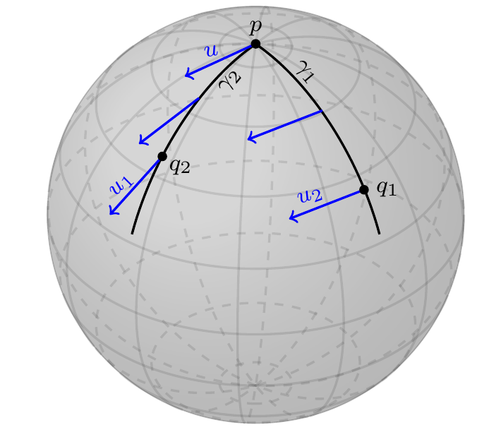{width=70%}
### Interactive: Parallel Transport on $\mathbb{S}^2$
The figure above shows transport around one specific geodesic triangle; the demo below lets you explore parallel transport along several curves on $\mathbb{S}^2$. Choose a curve from the dropdown, pick an initial tangent vector $v_0 \in T_{\gamma(0)}\mathbb{S}^2$ (direction and length), and drag the progress slider to transport it along the curve. Along a geodesic (equator, meridian, triangle edges) the angle between $V(t)$ and the velocity $\dot\gamma(t)$ stays constant; along a latitude circle or a loxodrome it changes. For a closed curve, $V$ generally does not return to $v_0$: the rotation after a full loop — the **holonomy** — equals the solid angle enclosed by the loop.
**Visual guide:**
- **Dashed purple curve** = the full curve $\gamma$; **solid purple segment** = the portion traversed so far
- **Red dot** = start point $\gamma(0)$; **purple dot** = current point $\gamma(t)$
- **Faint green arrow** = initial vector $v_0$ kept at $\gamma(0)$ for comparison
- **Bold green arrow** = transported vector $V(t)$ at $\gamma(t)$; **teal arrows** = $V$ at intermediate points
```{ojs}
//| label: fig-parallel-transport
//| fig-cap: "Interactive: Parallel transport of a tangent vector along a curve on the 2-sphere"
pt_curve_control = Inputs.select(new Map([
  ["Latitude circle (colatitude θ₀ = 45°)", "latitude"],
  ["Equator (geodesic)", "equator"],
  ["Meridian arc (geodesic)", "meridian"],
  ["Geodesic triangle (closed loop)", "triangle"],
  ["Loxodrome (constant bearing 70°)", "loxodrome"]
]), {value: "latitude", label: "Curve γ"})
pt_t_control = Inputs.range([0, 100], {step: 1, value: 60, label: "Transport progress (%)"})
pt_vang_control = Inputs.range([0, 360], {step: 5, value: 60, label: "Initial direction of v₀ (°)"})
pt_vlen_control = Inputs.range([0.2, 1.5], {step: 0.1, value: 0.8, label: "Initial length |v₀|"})
pt_rotY_control = Inputs.range([0, 360], {step: 10, value: 210, label: "Transport view azimuth °"})
pt_rotX_control = Inputs.range([-50, 50], {step: 5, value: 20, label: "Transport view elevation °"})
pt_curve = Generators.input(pt_curve_control)
pt_t = Generators.input(pt_t_control)
pt_vang = Generators.input(pt_vang_control)
pt_vlen = Generators.input(pt_vlen_control)
pt_rotY = Generators.input(pt_rotY_control)
pt_rotX = Generators.input(pt_rotX_control)

pt_controls_view = html`
<style>
  .pt-slider-grid { display:flex; flex-wrap:wrap; gap:6px 20px; width:100%; margin:0 0 12px; font:0.85em system-ui,sans-serif; container-type:inline-size; }
  .pt-slider-grid > * { flex:1 1 calc((100% - 40px)/3); min-width:0; margin:0; }
  .pt-slider-grid input[type="number"] { width:7.5rem !important; }
  .pt-s2-globe { display:block; width:100%; height:auto; }
  @container (max-width:700px) { .pt-slider-grid > * { flex-basis:calc((100% - 20px)/2); } }
  @container (max-width:480px) { .pt-slider-grid > * { flex-basis:100%; } }
</style>
<div class="pt-slider-grid">
  <div>${pt_curve_control}</div>
  <div>${pt_t_control}</div>
  <div>${pt_vang_control}</div>
  <div>${pt_vlen_control}</div>
  <div>${pt_rotY_control}</div>
  <div>${pt_rotX_control}</div>
</div>`

function runParallelTransportDemo(curveName, tPct, vAngDeg, vLen, rotYdeg, rotXdeg) {
  var D2R = Math.PI / 180;
  function dot3(a, b) { return a[0]*b[0] + a[1]*b[1] + a[2]*b[2]; }
  function cross3(a, b) { return [a[1]*b[2]-a[2]*b[1], a[2]*b[0]-a[0]*b[2], a[0]*b[1]-a[1]*b[0]]; }
  function norm3(a) { return Math.sqrt(dot3(a, a)); }
  function clamp1(x) { return Math.max(-1, Math.min(1, x)); }

  // Curve definitions: t in [0,1] -> unit vector on S²
  var curveLabel, closed = false, curveFn;
  if (curveName === "equator") {
    curveLabel = "Equator (geodesic)";
    closed = true;
    curveFn = function(t) {
      var ph = 2*Math.PI*t;
      return [Math.cos(ph), Math.sin(ph), 0];
    };
  } else if (curveName === "meridian") {
    curveLabel = "Meridian arc (geodesic)";
    var ph0 = 30*D2R;
    curveFn = function(t) {
      var th = (15 + 150*t)*D2R;
      return [Math.sin(th)*Math.cos(ph0), Math.sin(th)*Math.sin(ph0), Math.cos(th)];
    };
  } else if (curveName === "triangle") {
    curveLabel = "Geodesic triangle (closed loop)";
    closed = true;
    var Nv = [0, 0, 1], Av = [1, 0, 0], Bv = [0, 1, 0];
    function slerp(a, b, s) {
      var om = Math.acos(clamp1(dot3(a, b)));
      if (om < 1e-12) return a.slice();
      var wa = Math.sin((1-s)*om)/Math.sin(om), wb = Math.sin(s*om)/Math.sin(om);
      return [wa*a[0]+wb*b[0], wa*a[1]+wb*b[1], wa*a[2]+wb*b[2]];
    }
    curveFn = function(t) {
      if (t < 1/3) return slerp(Nv, Av, 3*t);
      if (t < 2/3) return slerp(Av, Bv, 3*t-1);
      return slerp(Bv, Nv, 3*t-2);
    };
  } else if (curveName === "loxodrome") {
    curveLabel = "Loxodrome (constant bearing 70°)";
    var tanB = Math.tan(70*D2R);
    var thMin = 25*D2R, thMax = 155*D2R;
    curveFn = function(t) {
      var th = thMax + (thMin-thMax)*t;
      var ph = tanB*Math.log(Math.tan(th/2)/Math.tan(thMax/2));
      return [Math.sin(th)*Math.cos(ph), Math.sin(th)*Math.sin(ph), Math.cos(th)];
    };
  } else {
    curveLabel = "Latitude circle (colatitude θ₀ = 45°)";
    closed = true;
    var th0 = 45*D2R;
    curveFn = function(t) {
      var ph = 2*Math.PI*t;
      return [Math.sin(th0)*Math.cos(ph), Math.sin(th0)*Math.sin(ph), Math.cos(th0)];
    };
  }

  // Sample the curve
  var N = 600, pts = [];
  for (var i = 0; i <= N; i++) pts.push(curveFn(i/N));

  // Initial vector in the local (eθ, eφ) frame at γ(0)
  var P0 = pts[0];
  var thP = Math.acos(clamp1(P0[2]));
  var phP = Math.atan2(P0[1], P0[0]);
  var eTh = [Math.cos(thP)*Math.cos(phP), Math.cos(thP)*Math.sin(phP), -Math.sin(thP)];
  var ePh = [-Math.sin(phP), Math.cos(phP), 0];
  var vAng = vAngDeg*D2R;
  var V0 = [
    vLen*(Math.cos(vAng)*eTh[0] + Math.sin(vAng)*ePh[0]),
    vLen*(Math.cos(vAng)*eTh[1] + Math.sin(vAng)*ePh[1]),
    vLen*(Math.cos(vAng)*eTh[2] + Math.sin(vAng)*ePh[2])
  ];

  // Parallel transport: march along the sampled points; each step rotates v
  // by the rotation taking pts[i-1] to pts[i] (Rodrigues' formula). This is
  // the exact transport along the joining geodesic arc, and converges to the
  // Levi-Civita parallel transport along the smooth curve as N grows.
  var vecs = new Array(N+1);
  vecs[0] = V0;
  var v = V0;
  for (var i = 1; i <= N; i++) {
    var a = pts[i-1], b = pts[i];
    var ax = cross3(a, b);
    var axn = norm3(ax);
    var nv = v;
    if (axn > 1e-12) {
      var ang = Math.atan2(axn, clamp1(dot3(a, b)));
      var k = [ax[0]/axn, ax[1]/axn, ax[2]/axn];
      var cA = Math.cos(ang), sA = Math.sin(ang);
      var kv = cross3(k, v);
      var kdv = dot3(k, v);
      nv = [
        v[0]*cA + kv[0]*sA + k[0]*kdv*(1-cA),
        v[1]*cA + kv[1]*sA + k[1]*kdv*(1-cA),
        v[2]*cA + kv[2]*sA + k[2]*kdv*(1-cA)
      ];
    }
    // numerical hygiene: re-project onto T_b S² and restore the length
    var dvb = dot3(nv, b);
    nv = [nv[0]-dvb*b[0], nv[1]-dvb*b[1], nv[2]-dvb*b[2]];
    var nvn = norm3(nv);
    if (nvn > 1e-12) nv = [nv[0]*vLen/nvn, nv[1]*vLen/nvn, nv[2]*vLen/nvn];
    vecs[i] = nv;
    v = nv;
  }

  // Current state
  var iT = Math.round(N*tPct/100);
  var curPt = pts[iT], curVec = vecs[iT];
  var curTh = Math.acos(clamp1(curPt[2]))/D2R;
  var curPh = ((Math.atan2(curPt[1], curPt[0])/D2R) + 360) % 360;

  // Angle between V(t) and the velocity γ̇(t)
  var iA = Math.max(0, iT-1), iB = Math.min(N, iT+1);
  var vel = [pts[iB][0]-pts[iA][0], pts[iB][1]-pts[iA][1], pts[iB][2]-pts[iA][2]];
  var dvl = dot3(vel, curPt);
  vel = [vel[0]-dvl*curPt[0], vel[1]-dvl*curPt[1], vel[2]-dvl*curPt[2]];
  var veln = norm3(vel);
  var angleVelDeg = null;
  if (veln > 1e-9) angleVelDeg = Math.acos(clamp1(dot3(vel, curVec)/(veln*vLen)))/D2R;

  // Intermediate arrow samples along the traversed portion
  var arrowSamples = [];
  if (iT > 1) {
    var step = Math.max(1, Math.floor(iT/14));
    for (var j = step; j < iT; j += step) arrowSamples.push({p: pts[j], v: vecs[j]});
  }

  // Rotation relative to the initial vector (holonomy when the loop closes)
  var rotVsInitDeg = null;
  if (closed && iT > 0) {
    var a0 = Math.atan2(dot3(V0, ePh), dot3(V0, eTh));
    var a1 = Math.atan2(dot3(curVec, ePh), dot3(curVec, eTh));
    rotVsInitDeg = (((a1-a0)/D2R) % 360 + 360) % 360;
  }

  // View rotation
  var ry = rotYdeg*D2R, rx = rotXdeg*D2R;
  function rotate(vv) {
    var x1 = vv[0]*Math.cos(ry) + vv[2]*Math.sin(ry), y1 = vv[1], z1 = -vv[0]*Math.sin(ry) + vv[2]*Math.cos(ry);
    return [x1, y1*Math.cos(rx) - z1*Math.sin(rx), y1*Math.sin(rx) + z1*Math.cos(rx)];
  }

  return {
    curve: pts, trajPts: pts.slice(0, iT+1),
    P0: P0, V0: V0, curPt: curPt, curVec: curVec,
    arrowSamples: arrowSamples,
    curveLabel: curveLabel, closed: closed,
    vLen: vLen, curNorm: norm3(curVec),
    angleVelDeg: angleVelDeg, rotVsInitDeg: rotVsInitDeg,
    curThetaDeg: curTh, curPhiDeg: curPh,
    rotate: rotate
  };
}

ptData = runParallelTransportDemo(pt_curve, pt_t, pt_vang, pt_vlen, pt_rotY, pt_rotX);

(() => {
const view = html`
<div style="font-family: system-ui, sans-serif;">

  <div style="display: flex; gap: 20px; flex-wrap: wrap;">

    <!-- Sphere + transported vector visualization -->
    <div style="flex: 0 0 calc(50% - 10px); min-width: 0;">
      <h4>Parallel Transport along γ on 𝕊²</h4>
      <svg class="pt-s2-globe" viewBox="0 0 420 420" role="img" aria-label="Sphere with a curve and a parallel transported tangent vector" style="border: 1px solid #dee2e6; border-radius: 4px; cursor: grab; touch-action: none; user-select: none; background: linear-gradient(180deg, #fbfdff 0%, #f5f8fb 100%);">
        <g transform="translate(210, 210)">
          ${(() => {
            var R = 175, parts = [];
            var res = ptData;

            function proj(v) {
              var rv = res.rotate(v);
              return {x: rv[0]*R, y: -rv[1]*R, z: rv[2]};
            }

            // Sphere wireframe
            for (var p = 0; p <= 18; p++) {
              var z = 1 - p*2/18;
              var r = Math.sqrt(Math.max(0, 1 - z*z));
              var d = '';
              for (var j = 0; j <= 120; j++) {
                var phi = j*2*Math.PI/120;
                var pt = proj([r*Math.cos(phi), r*Math.sin(phi), z]);
                d += (j===0?'M':'L')+' '+pt.x.toFixed(1)+' '+pt.y.toFixed(1);
              }
              parts.push('<path d="'+d+'" fill="none" stroke="#adb5bd" stroke-width="0.5" opacity="0.12"/>');
            }
            for (var m = 0; m < 24; m++) {
              var phi = m*Math.PI/12;
              var d = '';
              for (var j = 0; j <= 90; j++) {
                var theta = j*Math.PI/90;
                var pt = proj([Math.sin(theta)*Math.cos(phi), Math.sin(theta)*Math.sin(phi), Math.cos(theta)]);
                d += (j===0?'M':'L')+' '+pt.x.toFixed(1)+' '+pt.y.toFixed(1);
              }
              parts.push('<path d="'+d+'" fill="none" stroke="#adb5bd" stroke-width="0.5" opacity="0.12"/>');
            }
            parts.push('<circle cx="0" cy="0" r="'+R+'" fill="none" stroke="#dee2e6" stroke-width="1.2"/>');

            function pathFrom(points) {
              var d = '';
              for (var i = 0; i < points.length; i++) {
                var pt = proj(points[i]);
                d += (i===0?'M':'L')+' '+pt.x.toFixed(1)+' '+pt.y.toFixed(1);
              }
              return d;
            }

            // Full curve (dashed) and traversed portion (solid)
            parts.push('<path d="'+pathFrom(res.curve)+'" fill="none" stroke="#9775fa" stroke-width="1.1" stroke-dasharray="4,4" opacity="0.5"/>');
            if (res.trajPts.length > 1) {
              parts.push('<path d="'+pathFrom(res.trajPts)+'" fill="none" stroke="#7950f2" stroke-width="2.6"/>');
            }

            function drawArrow(base, vec, scl, color, w, op) {
              var tip = [base[0]+scl*vec[0], base[1]+scl*vec[1], base[2]+scl*vec[2]];
              var bP = proj(base), tP = proj(tip);
              var s = '<line x1="'+bP.x.toFixed(1)+'" y1="'+bP.y.toFixed(1)+'" x2="'+tP.x.toFixed(1)+'" y2="'+tP.y.toFixed(1)+'" stroke="'+color+'" stroke-width="'+w+'" stroke-linecap="round" opacity="'+op+'"/>';
              var vn = Math.sqrt(vec[0]*vec[0]+vec[1]*vec[1]+vec[2]*vec[2]);
              if (vn > 1e-9) {
                var vd = [vec[0]/vn, vec[1]/vn, vec[2]/vn];
                var ox = vd[1]*base[2]-vd[2]*base[1], oy = vd[2]*base[0]-vd[0]*base[2], oz = vd[0]*base[1]-vd[1]*base[0];
                var on = Math.sqrt(ox*ox+oy*oy+oz*oz);
                if (on > 1e-9) {
                  ox /= on; oy /= on; oz /= on;
                  var hl = Math.min(0.3*vn, 0.15), hw = Math.min(0.18*vn, 0.08);
                  var wb = [tip[0]-scl*hl*vd[0], tip[1]-scl*hl*vd[1], tip[2]-scl*hl*vd[2]];
                  var w1 = proj([wb[0]+scl*hw*ox, wb[1]+scl*hw*oy, wb[2]+scl*hw*oz]);
                  var w2 = proj([wb[0]-scl*hw*ox, wb[1]-scl*hw*oy, wb[2]-scl*hw*oz]);
                  s += '<polygon points="'+tP.x.toFixed(1)+','+tP.y.toFixed(1)+' '+w1.x.toFixed(1)+','+w1.y.toFixed(1)+' '+w2.x.toFixed(1)+','+w2.y.toFixed(1)+'" fill="'+color+'" opacity="'+op+'"/>';
                }
              }
              return s;
            }

            // Transported vector at intermediate points (teal)
            for (var ai = 0; ai < res.arrowSamples.length; ai++) {
              parts.push(drawArrow(res.arrowSamples[ai].p, res.arrowSamples[ai].v, 0.45, '#0ca678', 1.6, 0.85));
            }
            // Initial vector kept at the start (faint green) and current vector (bold green)
            parts.push(drawArrow(res.P0, res.V0, 0.45, '#2b8a3e', 2, 0.4));
            parts.push(drawArrow(res.curPt, res.curVec, 0.45, '#2b8a3e', 3, 1));

            var tipV = proj([res.curPt[0]+0.45*res.curVec[0], res.curPt[1]+0.45*res.curVec[1], res.curPt[2]+0.45*res.curVec[2]]);
            parts.push('<text x="'+(tipV.x+5).toFixed(0)+'" y="'+(tipV.y-6).toFixed(0)+'" font-size="11" fill="#2b8a3e" font-weight="bold">V(t)</text>');

            // Start and current points
            var p0P = proj(res.P0);
            parts.push('<circle cx="'+p0P.x.toFixed(1)+'" cy="'+p0P.y.toFixed(1)+'" r="5.5" fill="#e03131" stroke="#fff" stroke-width="1.5"/>');
            parts.push('<text x="'+(p0P.x+8).toFixed(0)+'" y="'+(p0P.y-7).toFixed(0)+'" font-size="12" fill="#e03131" font-weight="bold">γ(0)</text>');
            var pcP = proj(res.curPt);
            parts.push('<circle cx="'+pcP.x.toFixed(1)+'" cy="'+pcP.y.toFixed(1)+'" r="5" fill="#7950f2" stroke="#fff" stroke-width="1.5"/>');
            parts.push('<text x="'+(pcP.x+7).toFixed(0)+'" y="'+(pcP.y-6).toFixed(0)+'" font-size="11" fill="#7950f2" font-weight="bold">γ(t)</text>');

            return parts.join('\n');
          })()}
        </g>
        <g transform="translate(15, 385)">
          <circle cx="0" cy="0" r="4" fill="#e03131"/><text x="8" y="4" font-size="10" fill="#495057">γ(0) start</text>
          <line x1="85" y1="0" x2="100" y2="0" stroke="#7950f2" stroke-width="2.5"/><text x="104" y="4" font-size="10" fill="#495057">traversed γ</text>
          <line x1="180" y1="0" x2="195" y2="0" stroke="#0ca678" stroke-width="2"/><text x="199" y="4" font-size="10" fill="#495057">V along curve</text>
          <line x1="290" y1="0" x2="305" y2="0" stroke="#2b8a3e" stroke-width="2.5"/><text x="309" y="4" font-size="10" fill="#495057">V(t)</text>
        </g>
        <text x="210" y="412" text-anchor="middle" font-size="10" fill="#6c757d">Drag the sphere to rotate and tilt</text>
      </svg>
    </div>

    <!-- Right panel -->
    <div style="flex: 0 0 calc(50% - 10px); min-width: 0;">
      <div style="padding: 12px; background: #f8f9fa; border-radius: 6px; margin-bottom: 12px;">
        <table style="width: 100%; border-collapse: collapse; font-size: 0.9em;">
          <tr><td style="padding: 3px 8px;">Curve γ</td>
              <td style="padding: 3px 8px; text-align: right;">${ptData.curveLabel}</td></tr>
          <tr><td style="padding: 3px 8px;">Progress</td>
              <td style="padding: 3px 8px; text-align: right; font-family: monospace;">${pt_t}%</td></tr>
          <tr><td style="padding: 3px 8px;">Current point γ(t)</td>
              <td style="padding: 3px 8px; text-align: right; font-family: monospace;">θ=${ptData.curThetaDeg.toFixed(1)}°, φ=${ptData.curPhiDeg.toFixed(1)}°</td></tr>
          <tr><td style="padding: 3px 8px; color: #2b8a3e;">|v₀| at γ(0)</td>
              <td style="padding: 3px 8px; text-align: right; font-family: monospace;">${ptData.vLen.toFixed(2)}</td></tr>
          <tr><td style="padding: 3px 8px; color: #2b8a3e; font-weight: bold;">|V(t)| transported</td>
              <td style="padding: 3px 8px; text-align: right; font-family: monospace;">${ptData.curNorm.toFixed(4)}</td></tr>
          <tr><td colspan="2"><hr style="margin: 4px 0;"></td></tr>
          <tr><td style="padding: 3px 8px;">∠(V(t), γ̇(t))</td>
              <td style="padding: 3px 8px; text-align: right; font-family: monospace;">${(() => { return ptData.angleVelDeg === null ? "—" : ptData.angleVelDeg.toFixed(1)+"°"; })()}</td></tr>
          ${(() => {
            if (ptData.rotVsInitDeg === null) return "";
            var suffix = (pt_t >= 99.5 && ptData.closed) ? " (holonomy)" : "";
            return '<tr><td style="padding: 3px 8px; color: #e8590c; font-weight: bold;">Rotation vs v₀' + suffix + '</td>' +
              '<td style="padding: 3px 8px; text-align: right; font-family: monospace;">' + ptData.rotVsInitDeg.toFixed(1) + '°</td></tr>';
          })()}
        </table>
      </div>
    </div>
  </div>
</div>
`
return attachS2DragRotation(view, ".pt-s2-globe", "Transport view azimuth", "Transport view elevation", -50, 50, ptData, "pt");
})()
```
::: {.callout-tip appearance="simple" title="Key concepts visualized"}
- **Metric compatibility:** $|V(t)|$ stays equal to $|v_0|$ — parallel transport preserves lengths (and, for several vectors transported together, their mutual angles).
- **Geodesics:** along the equator, the meridian, and each edge of the triangle, the velocity $\dot\gamma$ is itself parallel, so $\angle\bigl(V(t), \dot\gamma(t)\bigr)$ stays constant along the curve.
- **Holonomy = curvature:** for the geodesic triangle at $t = 100\%$, $V$ returns rotated by exactly the enclosed area $\pi/2 = 90^\circ$ (the unit sphere has $K = +1$); for the latitude circle at $\theta_0 = 45^\circ$ the rotation equals the enclosed solid angle $2\pi(1 - \cos\theta_0) \approx 105.4^\circ$.
- Drag the sphere to view the transport from different angles.
:::
::: {.callout-note appearance="simple" collapse="true" title="Geodesics: Riemannian connection vs. metric-space definition"}
The notion of a geodesic exists in two guises — one differential-geometric, one metric — and understanding their relationship and differences is important.
**Riemannian (connection-based) definition.** A smooth curve $\gamma$ is a **geodesic** if it satisfies $\nabla_{\dot\gamma}\dot\gamma = 0$, i.e., its velocity is covariantly constant. This is a *second-order* differential condition that guarantees constant speed ($\frac{d}{dt}\|\dot\gamma\|^2 = 0$) and, via the first variation formula, local length-minimization. The exponential map $\exp_p(v) = \gamma_v(1)$ is built from this definition.
**Metric-space definition.** In a general metric space $(\mathcal{M},d)$, a curve $\gamma:I\to\mathcal M$ is a **constant-speed local geodesic** if there is a constant $c\ge0$ such that every $t\in I$ has a neighborhood on which
$$
d\bigl(\gamma(s),\gamma(s')\bigr)=c|s-s'|.
$$
This is a metric condition—no derivatives or connection are required—and it applies to nonsmooth spaces such as Wasserstein and $\operatorname{CAT}(\kappa)$ spaces. A **globally minimizing geodesic segment** satisfies the same equality for every pair $s,s'\in I$. A locally geodesic curve need not minimize between distant endpoints.
**How they relate.**
| Aspect | Riemannian geodesic ($\nabla_{\dot\gamma}\dot\gamma=0$) | Metric geodesic (local length-minimizer) |
|---|---|---|
| Requires | Smooth manifold + connection | Only a metric $d$ |
| Form | Second-order ODE | Metric/variational condition |
| Constant speed | Automatic | By parameterization convention |
| Local minimizer | Yes | Yes (definition) |
| Uniqueness from point + initial velocity | Unique maximal solution for a smooth connection | No velocity datum is intrinsic; endpoint geodesics need not be unique |
| Existence between two points | Connected complete manifolds (Hopf–Rinow) | Geodesic metric spaces |
**Local equivalence on Riemannian manifolds.** On a Riemannian manifold $(\mathcal{M}, g)$ with the Levi–Civita connection, the two definitions coincide: every solution to $\nabla_{\dot\gamma}\dot\gamma = 0$ is locally length-minimizing, and every locally length-minimizing curve parameterized proportionally to arc length is a solution to $\nabla_{\dot\gamma}\dot\gamma = 0$. However, globally, a geodesic on manifolds may fail to minimize length between its endpoints (e.g., a great circle on the sphere).
:::
::: {#thm-hopf-rinow .theorem title="Hopf–Rinow"}
On a connected Riemannian manifold, the following are equivalent: (i) metric completeness, (ii) geodesic completeness, (iii) for every $p$, $\exp_p$ is defined on all of $T_p\mathcal{M}$, and (iv) every closed and bounded subset is compact. Any of these implies that any two points can be joined by a minimizing geodesic [@Lee2018].
:::
### Curvature
The **Riemann curvature tensor** is
$$
R(U, V)W = \nabla_U\nabla_V W - \nabla_V\nabla_U W - \nabla_{[U,V]}W.
$$
For linearly independent $u, v \in T_p\mathcal{M}$, the **sectional curvature** of $\Pi = \operatorname{span}\{u, v\}$ is
$$
\mathfrak{K}_p(u, v) = \frac{g_p(R(u, v)v, u)}{g_p(u, u)g_p(v, v) - g_p(u, v)^2}.
$$
With this convention, the unit sphere has sectional curvature $+1$, Euclidean space has curvature $0$, and unit hyperbolic space has curvature $-1$.
::: {#thm-sectional-alexandrov .theorem title="Sectional curvature and comparison geometry"}
- Sectional curvature $\le \kappa$ is equivalent to being locally $\mathrm{CAT}(\kappa)$.
- Sectional curvature $\ge \kappa$ is equivalent to having local Alexandrov curvature bounded below by $\kappa$.
- Complete, simply connected, sectional curvature $\le 0$ implies global $\mathrm{CAT}(0)$ (a Hadamard manifold).
:::
A **Hadamard manifold** is complete, simply connected, with nonpositive sectional curvature. On such a manifold, any two points have a unique minimizing geodesic and $x\mapsto d^2(x,y)$ is strongly geodesically convex. Consequently, every probability distribution with finite second moment has a unique Fréchet mean [@Bridson1999; @Sturm2003].
## Exponential and Logarithmic Maps
::: {#def-exp-log .definition title="Exponential and logarithmic maps"}
For $p\in\mathcal M$ and $v\in T_p\mathcal M$, let $\gamma_v$ be the maximal geodesic with $\gamma_v(0)=p$ and $\dot\gamma_v(0)=v$. Whenever $\gamma_v$ is defined at time $1$, the **exponential map** is $\exp_p(v)=\gamma_v(1)$. Thus $\exp_p$ is defined on an open subset of $T_p\mathcal M$ containing $0$; if $\mathcal M$ is geodesically complete, its domain is all of $T_p\mathcal M$. On a normal neighborhood of $p$, the local inverse of $\exp_p$ is the **logarithmic map** $\log_p$.
:::
Assume $\mathcal{M}$ is complete. Along a unit-speed geodesic from $p$, the **cut time** is the supremum of the times up to which the segment starting at $p$ remains minimizing; when finite, the endpoint at that time is a cut point. The union of all such endpoints is $\operatorname{Cut}(p)$. There is an open, star-shaped injectivity domain $\mathcal{I}_p\subset T_p\mathcal{M}$ containing $0$ such that
$$
\exp_p\big|_{\mathcal{I}_p}:\mathcal{I}_p\longrightarrow \mathcal{M}\setminus\operatorname{Cut}(p)
$$
is a diffeomorphism. Its inverse is the single-valued map $\log_p$ on $\mathcal{M}\setminus\operatorname{Cut}(p)$. On the unit sphere, $\operatorname{Cut}(p)=\{-p\}$.
::: {.callout-note title="Example: $\exp$ and $\log$ in Euclidean space"}
Let $\mathcal{M} = \mathbb{R}^d$ with the standard Euclidean metric $g_p(u,v) = u^\top v$. Geodesics are straight lines $\gamma(t) = p + tv$, so the exponential map is simply addition:
$$
\exp_p(v) = \gamma_v(1) = p + v, \qquad v \in T_p\mathbb{R}^d \cong \mathbb{R}^d.
$$
The logarithmic map is the difference vector:
$$
\log_p(q) = q - p, \qquad q \in \mathbb{R}^d.
$$
Because geodesics are globally minimizing, the cut locus is empty ($\operatorname{Cut}(p) = \varnothing$), and $\exp_p$, $\log_p$ are global diffeomorphisms — a stark contrast to curved manifolds like $\mathbb{S}^2$, where the cut locus forces these maps to be only local inverses. This Euclidean baseline is what general Riemannian geometry reduces to when curvature vanishes.
:::
**Interactive Exploration: Exponential and Logarithmic Maps on $\mathbb{S}^2$.**
The exponential map $\exp_p(v)$ sends a tangent vector $v \in T_p\mathcal{M}$ to the point reached by following the geodesic with initial velocity $v$ for unit time. The logarithmic map $\log_p(q)$ is its local inverse: it returns the tangent vector at $p$ whose geodesic reaches $q$. This demo visualizes both maps simultaneously, along with the fundamental identity $\exp_p(\log_p(q)) = q$.
**Visual guide:**
- **Red dot** = base point $p$
- **Green arrow** = tangent vector $v$ (exp map input)
- **Purple dot** = $\exp_p(v)$ (exp map output)
- **Blue dot** = target point $q$ (log map input)
- **Orange arrow** = $\log_p(q)$ (log map output)
- **Dashed curves** = geodesics from $p$
- **Orange plane** = tangent space $T_p\mathbb{S}^2$
The tangent arrows are rescaled when necessary so they remain inside the display; the tables report their true norms.
```{ojs}
//| label: fig-exp-log-map
//| fig-cap: "Interactive: Exponential and logarithmic maps on the 2-sphere"
el_th_control = Inputs.range([1, 179], {step: 1, value: 35, label: "Base point θ (colatitude °)"})
el_ph_control = Inputs.range([0, 360], {step: 5, value: 70, label: "Base point φ (longitude °)"})
el_vang_control = Inputs.range([0, 360], {step: 10, value: 60, label: "Tangent direction (exp input) °"})
el_vlen_control = Inputs.range([0.2, 4.2], {step: 0.1, value: 1.6, label: "Tangent vector |v| (exp input)"})
el_qth_control = Inputs.range([0, 180], {step: 1, value: 110, label: "Target q θ (log input) °"})
el_qph_control = Inputs.range([0, 360], {step: 5, value: 200, label: "Target q φ (log input) °"})
el_rotY_control = Inputs.range([0, 360], {step: 10, value: 200, label: "Exp/log view azimuth °"})
el_rotX_control = Inputs.range([-50, 50], {step: 5, value: 20, label: "Exp/log view elevation °"})
el_th = Generators.input(el_th_control)
el_ph = Generators.input(el_ph_control)
el_vang = Generators.input(el_vang_control)
el_vlen = Generators.input(el_vlen_control)
el_qth = Generators.input(el_qth_control)
el_qph = Generators.input(el_qph_control)
el_rotY = Generators.input(el_rotY_control)
el_rotX = Generators.input(el_rotX_control)

el_controls_view = html`
<style>
  .el-slider-grid { display:flex; flex-wrap:wrap; gap:6px 20px; width:100%; margin:0 0 12px; font:0.85em system-ui,sans-serif; container-type:inline-size; }
  .el-slider-grid > * { flex:1 1 calc((100% - 40px)/3); min-width:0; margin:0; }
  .el-slider-grid input[type="number"] { width:7.5rem !important; }
  .explog-s2-globe { display:block; width:100%; height:auto; }
  @container (max-width:700px) { .el-slider-grid > * { flex-basis:calc((100% - 20px)/2); } }
  @container (max-width:480px) { .el-slider-grid > * { flex-basis:100%; } }
</style>
<div class="el-slider-grid">
  <div>${el_th_control}</div>
  <div>${el_ph_control}</div>
  <div>${el_vang_control}</div>
  <div>${el_vlen_control}</div>
  <div>${el_qth_control}</div>
  <div>${el_qph_control}</div>
  <div>${el_rotY_control}</div>
  <div>${el_rotX_control}</div>
</div>`

function runExpLogDemo(pThDeg, pPhDeg, vAngDeg, vLen, qThDeg, qPhDeg, rotYdeg, rotXdeg) {
  var pTh = pThDeg * Math.PI / 180;
  var pPh = pPhDeg * Math.PI / 180;
  var vAng = vAngDeg * Math.PI / 180;
  var qTh = qThDeg * Math.PI / 180;
  var qPh = qPhDeg * Math.PI / 180;

  // Base point
  var P = [Math.sin(pTh)*Math.cos(pPh), Math.sin(pTh)*Math.sin(pPh), Math.cos(pTh)];
  // Target point q
  var Q = [Math.sin(qTh)*Math.cos(qPh), Math.sin(qTh)*Math.sin(qPh), Math.cos(qTh)];

  // Tangent basis at P
  var eTheta = [Math.cos(pTh)*Math.cos(pPh), Math.cos(pTh)*Math.sin(pPh), -Math.sin(pTh)];
  var ePhi = [-Math.sin(pPh), Math.cos(pPh), 0];

  // Tangent vector V from user input
  var V = [
    vLen * (Math.cos(vAng)*eTheta[0] + Math.sin(vAng)*ePhi[0]),
    vLen * (Math.cos(vAng)*eTheta[1] + Math.sin(vAng)*ePhi[1]),
    vLen * (Math.cos(vAng)*eTheta[2] + Math.sin(vAng)*ePhi[2])
  ];
  var Vnorm = Math.sqrt(V[0]*V[0]+V[1]*V[1]+V[2]*V[2]);

  // Helper: exp map on S²
  function expS2(base, vec) {
    var nv = Math.sqrt(vec[0]*vec[0]+vec[1]*vec[1]+vec[2]*vec[2]);
    if (nv < 1e-12) return [base[0], base[1], base[2]];
    var c = Math.cos(nv), s = Math.sin(nv);
    return [c*base[0]+s*vec[0]/nv, c*base[1]+s*vec[1]/nv, c*base[2]+s*vec[2]/nv];
  }

  // Helper: log map on S²
  function logS2(base, target) {
    var dot = base[0]*target[0]+base[1]*target[1]+base[2]*target[2];
    dot = Math.max(-1, Math.min(1, dot));
    var dist = Math.acos(dot);
    if (dist < 1e-12) return [0, 0, 0];
    if (Math.PI - dist < 1e-7) return null; // antipode: no single-valued log
    // Compute tangent direction: project target onto tangent plane
    var proj = [target[0]-dot*base[0], target[1]-dot*base[1], target[2]-dot*base[2]];
    var nProj = Math.sqrt(proj[0]*proj[0]+proj[1]*proj[1]+proj[2]*proj[2]);
    if (nProj < 1e-12) return [0, 0, 0];
    return [dist*proj[0]/nProj, dist*proj[1]/nProj, dist*proj[2]/nProj];
  }

  // exp_P(V)
  var expV = expS2(P, V);
  // log_P(Q)
  var logQ = logS2(P, Q);
  var logDefined = logQ !== null;
  var logNorm = logDefined ? Math.sqrt(logQ[0]*logQ[0]+logQ[1]*logQ[1]+logQ[2]*logQ[2]) : null;
  // exp_P(log_P(Q)) recovers Q only where the single-valued log exists
  var expLogQ = logDefined ? expS2(P, logQ) : null;
  var expDot = Math.max(-1, Math.min(1, P[0]*expV[0]+P[1]*expV[1]+P[2]*expV[2]));
  var expDistance = Math.acos(expDot);

  // Geodesic for exp (P -> expV)
  var nExpPts = 30;
  var geodExp = [];
  for (var i = 0; i <= nExpPts; i++) {
    var t = i/nExpPts;
    geodExp.push(expS2(P, [t*V[0], t*V[1], t*V[2]]));
  }
  // Geodesic for log (P -> Q)
  var nLogPts = 30;
  var geodLog = [];
  if (logDefined) {
    for (var i = 0; i <= nLogPts; i++) {
      geodLog.push(expS2(P, [i/nLogPts*logQ[0], i/nLogPts*logQ[1], i/nLogPts*logQ[2]]));
    }
  }

  // Tangent plane grid at P
  var tgGrid = [];
  var gridExt = 0.7, nGrid = 9;
  for (var i = 0; i < nGrid; i++) {
    for (var j = 0; j < nGrid; j++) {
      var a = (i/(nGrid-1) - 0.5) * 2 * gridExt;
      var b = (j/(nGrid-1) - 0.5) * 2 * gridExt;
      tgGrid.push([P[0]+a*eTheta[0]+b*ePhi[0], P[1]+a*eTheta[1]+b*ePhi[1], P[2]+a*eTheta[2]+b*ePhi[2]]);
    }
  }

  // Rotation
  var ry = rotYdeg*Math.PI/180, rx = rotXdeg*Math.PI/180;
  function rotate(v) {
    var x1 = v[0]*Math.cos(ry)+v[2]*Math.sin(ry), y1 = v[1], z1 = -v[0]*Math.sin(ry)+v[2]*Math.cos(ry);
    return [x1, y1*Math.cos(rx)-z1*Math.sin(rx), y1*Math.sin(rx)+z1*Math.cos(rx)];
  }

  return {
    P: P, Q: Q, V: V, Vnorm: Vnorm, expV: expV, expDistance: expDistance,
    logQ: logQ, logNorm: logNorm, logDefined: logDefined, expLogQ: expLogQ,
    geodExp: geodExp, geodLog: geodLog,
    tgGrid: tgGrid, nGrid: nGrid, eTheta: eTheta, ePhi: ePhi,
    rotate: rotate
  };
}

elData = runExpLogDemo(el_th, el_ph, el_vang, el_vlen, el_qth, el_qph, el_rotY, el_rotX);

(() => {
const view = html`
<div style="font-family: system-ui, sans-serif; width: 100%;">

  <div style="display: flex; gap: 20px; flex-wrap: wrap;">

    <!-- Sphere visualization -->
    <div style="flex: 1 1 0; min-width: 0;">
      <h4>exp<sub>p</sub> and log<sub>p</sub> on 𝕊²</h4>
      <svg class="explog-s2-globe" viewBox="0 0 430 430" role="img" aria-label="Exponential and logarithmic maps on the sphere" style="border: 1px solid #dee2e6; border-radius: 4px; cursor: grab; touch-action: none; user-select: none; background: linear-gradient(180deg, #fbfdff 0%, #f5f8fb 100%);">
        <g transform="translate(215, 215)">
          ${(() => {
            var R = 180, parts = [];
            var res = elData;

            function proj(v) {
              var rv = res.rotate(v);
              return {x: rv[0]*R, y: -rv[1]*R, z: rv[2]};
            }

            // Sphere wireframe
            for (var p = 0; p <= 18; p++) {
              var z = 1 - p*2/18, r = Math.sqrt(Math.max(0, 1 - z*z));
              var d = '';
              for (var j = 0; j <= 120; j++) {
                var phi = j*2*Math.PI/120, pt = proj([r*Math.cos(phi), r*Math.sin(phi), z]);
                d += (j===0?'M':'L')+' '+pt.x.toFixed(1)+' '+pt.y.toFixed(1);
              }
              parts.push('<path d="'+d+'" fill="none" stroke="#adb5bd" stroke-width="0.5" opacity="0.12"/>');
            }
            for (var m = 0; m < 24; m++) {
              var phi = m*Math.PI/12, d = '';
              for (var j = 0; j <= 90; j++) {
                var theta = j*Math.PI/90, pt = proj([Math.sin(theta)*Math.cos(phi), Math.sin(theta)*Math.sin(phi), Math.cos(theta)]);
                d += (j===0?'M':'L')+' '+pt.x.toFixed(1)+' '+pt.y.toFixed(1);
              }
              parts.push('<path d="'+d+'" fill="none" stroke="#adb5bd" stroke-width="0.5" opacity="0.12"/>');
            }
            parts.push('<circle cx="0" cy="0" r="'+R+'" fill="none" stroke="#dee2e6" stroke-width="1.2"/>');

            // Tangent plane grid
            for (var i = 0; i < res.nGrid; i++) {
              var dRow = '';
              for (var j = 0; j < res.nGrid; j++) {
                var pt = proj(res.tgGrid[i*res.nGrid+j]);
                dRow += (j===0?'M':'L')+' '+pt.x.toFixed(1)+' '+pt.y.toFixed(1);
              }
              parts.push('<path d="'+dRow+'" fill="none" stroke="#f08c00" stroke-width="0.3" opacity="0.15"/>');
            }
            for (var j = 0; j < res.nGrid; j++) {
              var dCol = '';
              for (var i = 0; i < res.nGrid; i++) {
                var pt = proj(res.tgGrid[i*res.nGrid+j]);
                dCol += (i===0?'M':'L')+' '+pt.x.toFixed(1)+' '+pt.y.toFixed(1);
              }
              parts.push('<path d="'+dCol+'" fill="none" stroke="#f08c00" stroke-width="0.3" opacity="0.15"/>');
            }

            // Geodesic from P toward expV (exp map: purple)
            var gExpPath = '';
            for (var gi = 0; gi < res.geodExp.length; gi++) {
              var pt = proj(res.geodExp[gi]);
              gExpPath += (gi===0?'M':'L')+' '+pt.x.toFixed(1)+' '+pt.y.toFixed(1);
            }
            parts.push('<path d="'+gExpPath+'" fill="none" stroke="#7950f2" stroke-width="2.5" stroke-dasharray="8,4"/>');

            // Minimizing geodesic from P to Q where the single-valued log exists
            if (res.logDefined) {
              var gLogPath = '';
              for (var gi = 0; gi < res.geodLog.length; gi++) {
                var pt = proj(res.geodLog[gi]);
                gLogPath += (gi===0?'M':'L')+' '+pt.x.toFixed(1)+' '+pt.y.toFixed(1);
              }
              parts.push('<path d="'+gLogPath+'" fill="none" stroke="#f08c00" stroke-width="2" stroke-dasharray="5,4"/>');
            }

            // Tangent vector V (green arrow from P)
            var pP = proj(res.P);
            var vScale = 0.55/Math.max(1, res.Vnorm);
            var vEnd = [res.P[0]+vScale*res.V[0], res.P[1]+vScale*res.V[1], res.P[2]+vScale*res.V[2]];
            var vdP = proj(vEnd);
            parts.push('<line x1="'+pP.x.toFixed(1)+'" y1="'+pP.y.toFixed(1)+'" x2="'+vdP.x.toFixed(1)+'" y2="'+vdP.y.toFixed(1)+'" stroke="#2b8a3e" stroke-width="3" stroke-linecap="round"/>');
            parts.push('<text x="'+(vdP.x+5).toFixed(0)+'" y="'+(vdP.y-7).toFixed(0)+'" font-size="11" fill="#2b8a3e" font-weight="bold">v</text>');

            // Log_P(Q) vector (orange arrow from P), absent at the antipode
            if (res.logDefined) {
              var logScale = 0.55/Math.max(1, res.logNorm);
              var logQend = [res.P[0]+logScale*res.logQ[0], res.P[1]+logScale*res.logQ[1], res.P[2]+logScale*res.logQ[2]];
              var lqP = proj(logQend);
              parts.push('<line x1="'+pP.x.toFixed(1)+'" y1="'+pP.y.toFixed(1)+'" x2="'+lqP.x.toFixed(1)+'" y2="'+lqP.y.toFixed(1)+'" stroke="#f08c00" stroke-width="2.5" stroke-linecap="round"/>');
              parts.push('<text x="'+(lqP.x+5).toFixed(0)+'" y="'+(lqP.y-7).toFixed(0)+'" font-size="11" fill="#f08c00" font-weight="bold">logₚ(q)</text>');
            }

            // expV point
            var expVP = proj(res.expV);
            parts.push('<circle cx="'+expVP.x.toFixed(1)+'" cy="'+expVP.y.toFixed(1)+'" r="5" fill="#7950f2" stroke="#fff" stroke-width="1.5"/>');
            parts.push('<text x="'+(expVP.x+6).toFixed(0)+'" y="'+(expVP.y-6).toFixed(0)+'" font-size="11" fill="#7950f2" font-weight="bold">expₚ(v)</text>');

            // Q point
            var qP = proj(res.Q);
            parts.push('<circle cx="'+qP.x.toFixed(1)+'" cy="'+qP.y.toFixed(1)+'" r="5" fill="#1971c2" stroke="#fff" stroke-width="1.5"/>');
            parts.push('<text x="'+(qP.x+6).toFixed(0)+'" y="'+(qP.y-6).toFixed(0)+'" font-size="11" fill="#1971c2" font-weight="bold">q</text>');

            // Base point P
            parts.push('<circle cx="'+pP.x.toFixed(1)+'" cy="'+pP.y.toFixed(1)+'" r="5.5" fill="#e03131" stroke="#fff" stroke-width="1.5"/>');
            parts.push('<text x="'+(pP.x+8).toFixed(0)+'" y="'+(pP.y-8).toFixed(0)+'" font-size="12" fill="#e03131" font-weight="bold">p</text>');

            return parts.join('\n');
          })()}
        </g>
        <g transform="translate(15, 395)">
          <circle cx="0" cy="0" r="4" fill="#e03131"/><text x="8" y="4" font-size="9" fill="#495057">p (base)</text>
          <line x1="68" y1="0" x2="80" y2="0" stroke="#2b8a3e" stroke-width="2.5"/><text x="84" y="4" font-size="9" fill="#495057">v (exp input)</text>
          <circle cx="188" cy="0" r="4" fill="#7950f2"/><text x="196" y="4" font-size="9" fill="#495057">expₚ(v)</text>
          <circle cx="298" cy="0" r="4" fill="#1971c2"/><text x="306" y="4" font-size="9" fill="#495057">q (log input)</text>
          <line x1="68" y1="12" x2="80" y2="12" stroke="#f08c00" stroke-width="2"/><text x="84" y="16" font-size="9" fill="#495057">logₚ(q)</text>
        </g>
        <text x="215" y="422" text-anchor="middle" font-size="10" fill="#6c757d">Drag the sphere to rotate and tilt</text>
      </svg>
    </div>

    <!-- Right panel: stats -->
    <div style="flex: 1 1 0; min-width: 0;">
      <div style="padding: 12px; background: #f8f9fa; border-radius: 6px; margin-bottom: 12px;">
        <h4 style="margin-top: 0;">Exponential Map</h4>
        <table style="width: 100%; border-collapse: collapse; font-size: 0.85em;">
          <tr><td style="padding: 3px 8px;">v = tangent vector at p</td>
              <td style="padding: 3px 8px; text-align: right; font-family: monospace;">|v| = ${elData.Vnorm.toFixed(3)}</td></tr>
          <tr><td style="padding: 3px 8px; color: #7950f2;">exp<sub>p</sub>(v)</td>
              <td style="padding: 3px 8px; text-align: right; font-family: monospace;">(${elData.expV[0].toFixed(3)}, ${elData.expV[1].toFixed(3)}, ${elData.expV[2].toFixed(3)})</td></tr>
          <tr><td style="padding: 3px 8px;">geodesic segment length</td>
              <td style="padding: 3px 8px; text-align: right; font-family: monospace;">${elData.Vnorm.toFixed(3)}</td></tr>
          <tr><td style="padding: 3px 8px;">d(p, exp<sub>p</sub>(v))</td>
              <td style="padding: 3px 8px; text-align: right; font-family: monospace;">${elData.expDistance.toFixed(3)}${elData.Vnorm <= Math.PI ? " = |v|" : " < |v| (wrapped)"}</td></tr>
        </table>
      </div>

      <div style="padding: 12px; background: #f8f9fa; border-radius: 6px; margin-bottom: 12px;">
        <h4 style="margin-top: 0;">Logarithmic Map</h4>
        <table style="width: 100%; border-collapse: collapse; font-size: 0.85em;">
          <tr><td style="padding: 3px 8px; color: #f08c00;">log<sub>p</sub>(q)</td>
              <td style="padding: 3px 8px; text-align: right; font-family: monospace; color:${elData.logDefined ? "#212529" : "#c92a2a"};">${elData.logDefined ? "|w| = "+elData.logNorm.toFixed(3) : "undefined at q = −p"}</td></tr>
          <tr><td style="padding: 3px 8px;">d(p, q)</td>
              <td style="padding: 3px 8px; text-align: right; font-family: monospace;">${(() => { var dot=elData.P[0]*elData.Q[0]+elData.P[1]*elData.Q[1]+elData.P[2]*elData.Q[2]; dot=Math.max(-1,Math.min(1,dot)); return (Math.acos(dot)*180/Math.PI).toFixed(2); })()}° = ${(() => { var dot=elData.P[0]*elData.Q[0]+elData.P[1]*elData.Q[1]+elData.P[2]*elData.Q[2]; dot=Math.max(-1,Math.min(1,dot)); return Math.acos(dot).toFixed(3); })()} rad</td></tr>
        </table>
      </div>
    </div>
  </div>
</div>
`
return attachS2DragRotation(view, ".explog-s2-globe", "Exp/log view azimuth", "Exp/log view elevation", -50, 50, elData, "explog");
})()
```
```{ojs}
html`
<div class="callout callout-style-default callout-note callout-titled">
  <div class="callout-header d-flex align-content-center">
    <div class="callout-icon-container">
      <i class="callout-icon"></i>
    </div>
    <div class="callout-title-container flex-fill">
      Inverse relationship: exp∘log = id (away from the cut locus)
    </div>
  </div>
  <div class="callout-body-container callout-body">
    <table style="width: 100%; border-collapse: collapse; font-size: 0.85em; margin-top: 4px;">
      <tr><td style="padding: 3px 8px;">exp<sub>p</sub>(log<sub>p</sub>(q))</td>
          <td style="padding: 3px 8px; text-align: right; font-family: monospace;">${elData.logDefined ? "("+elData.expLogQ[0].toFixed(3)+", "+elData.expLogQ[1].toFixed(3)+", "+elData.expLogQ[2].toFixed(3)+")" : "undefined"}</td></tr>
      <tr><td style="padding: 3px 8px;">Q (original target)</td>
          <td style="padding: 3px 8px; text-align: right; font-family: monospace;">(${elData.Q[0].toFixed(3)}, ${elData.Q[1].toFixed(3)}, ${elData.Q[2].toFixed(3)})</td></tr>
      <tr><td style="padding: 3px 8px; font-weight: bold;">‖exp<sub>p</sub>(log<sub>p</sub>(q)) − q‖</td>
          <td style="padding: 3px 8px; text-align: right; font-family: monospace; font-weight: bold;">${(() => { if (!elData.logDefined) return "undefined"; var d0=elData.expLogQ[0]-elData.Q[0], d1=elData.expLogQ[1]-elData.Q[1], d2=elData.expLogQ[2]-elData.Q[2]; return Math.sqrt(d0*d0+d1*d1+d2*d2).toExponential(2); })()}</td></tr>
    </table>
    <p style="margin: 8px 0 0 0; font-size: 0.85em; color:${elData.logDefined ? "#495057" : "#c92a2a"};">
      ${elData.logDefined
        ? "The near-zero residual confirms expₚ(logₚ(q)) = q away from the cut locus. This identity underlies gradₓ d²(x,y) = −2 logₓ(y)."
        : "Here q = −p is the cut point. Infinitely many length-π tangent vectors exponentiate to q, so no single-valued logₚ(q) exists and the inverse expression is undefined."}
    </p>
  </div>
</div>
`
```
::: {.callout-tip title="Try these experiments"}
- **Move q to coincide with $\exp_p(v)$:** When $|v|<\pi$, set q's coordinates to match $\exp_p(v)$ and observe that $\log_p(q)$ recovers $v$. For $|v|>\pi$, the displayed log is instead the shorter tangent vector to the same endpoint.
- **Move q to the antipodal point of p:** Set $\theta_q = 180° - \theta_p$, $\phi_q = \phi_p + 180°$. This is the cut locus of $p$ on $\mathbb{S}^2$, where $\log_p(q)$ is undefined (any direction gives the same distance $\pi$).
- **Vary the tangent vector length:** As $|v|$ approaches $\pi$, $\exp_p(v)$ approaches the antipodal point. For $|v| > \pi$, the geodesic segment wraps around and is no longer minimizing; compare its length with the intrinsic distance in the table.
- **Compare exp and log directions:** The green arrow (exp input) and orange arrow (log output) trace different geodesics — one toward $\exp_p(v)$ and one toward $q$. When they align, $\exp_p(v)$ and $q$ lie on the same geodesic ray from $p$.
:::
## Key Takeaways
- **Smooth manifolds** are spaces locally modeled on $\mathbb{R}^m$ with smooth coordinate transitions. An **atlas** is a collection of charts covering the manifold; stereographic projections from the north and south poles form an atlas for $\mathbb{S}^2$.
- The **tangent space** $T_p\mathcal{M}$ is a vector space of dimension $\dim\mathcal{M}$ attached to each point $p$, with a basis induced by any coordinate chart. Tangent vectors are velocities of curves through $p$.
- **Riemannian metrics** endow each tangent space with an inner product, defining length, distance, and geodesics.
- The **exponential map** $\exp_p(v)$ sends tangent vectors to manifold points along geodesics; its local inverse is the **logarithmic map** $\log_p(q)$. On $\mathbb{S}^2$, $\exp_p(v) = \cos(|v|)p + \sin(|v|)v/|v|$.
- **Sectional curvature** controls geodesic comparison: nonpositive curvature (Hadamard) guarantees convexity and unique Fréchet means; positive curvature (spheres) can produce multiple means.
- The **SPD cone** with affine-invariant or log-Euclidean metric and the **sphere** are two recurring Riemannian manifolds in data analysis.
## Exercises
1. **Stereographic transition.** Compute the transition map between the north-pole and south-pole stereographic charts on $\mathbb{S}^2$ and verify it is smooth. <a href="javascript:void(0)" onclick="showSolution('l15-sol-1')" class="solution-link">📝 Show Solution</a>
2. **SPD exponential.** Verify that $\mathrm{Exp}^{\mathrm{AI}}_\Sigma(U) = \Sigma^{1/2}\exp(\Sigma^{-1/2}U\Sigma^{-1/2})\Sigma^{1/2}$ satisfies $\mathrm{Exp}^{\mathrm{AI}}_\Sigma(0) = \Sigma$ and $\frac{d}{dt}|_{t=0}\mathrm{Exp}^{\mathrm{AI}}_\Sigma(tU) = U$. <a href="javascript:void(0)" onclick="showSolution('l15-sol-2')" class="solution-link">📝 Show Solution</a>
3. **Gradient formula on the circle.** For $\mathbb{S}^1$ with the arc-length metric, compute $\nabla d^2(\theta, \phi)$ explicitly and verify $\nabla d^2(\theta,\phi) = -2\log_\theta(\phi)$. <a href="javascript:void(0)" onclick="showSolution('l15-sol-3')" class="solution-link">📝 Show Solution</a>
4. **Hadamard vs. sphere.** Explain why a probability distribution with finite second moment has a unique Fréchet mean on a Hadamard manifold but may have multiple means on a sphere. Give a concrete counterexample on $\mathbb{S}^2$. <a href="javascript:void(0)" onclick="showSolution('l15-sol-4')" class="solution-link">📝 Show Solution</a>
<style>
.solution-link { font-size: 0.9em; text-decoration: none; white-space: nowrap; margin-left: 0.3em; }
.solution-link:hover { text-decoration: underline; }
.solution-dialog { padding: 0; max-width: 720px; }
.solution-dialog-header { display: flex; justify-content: space-between; align-items: flex-start; border-bottom: 1px solid #dee2e6; padding: 1.25rem 1.5rem 1rem; background: #f8f9fa; border-radius: 8px 8px 0 0; }
.solution-dialog-header h4 { margin: 0; font-size: 1.15rem; }
.solution-dialog-close { background: none; border: 1px solid #adb5bd; border-radius: 4px; padding: 0.2rem 0.75rem; cursor: pointer; font-size: 0.9rem; color: #495057; white-space: nowrap; flex-shrink: 0; }
.solution-dialog-close:hover { background: #e9ecef; }
.solution-original { padding: 1rem 1.5rem; background: #f1f3f5; border-left: 4px solid #868e96; margin: 1rem 1.5rem; border-radius: 4px; font-size: 0.95rem; }
.solution-answer { padding: 0.5rem 1.5rem 1.5rem; }
.solution-answer strong { color: #2b8a3e; }
dialog { border: none; border-radius: 8px; box-shadow: 0 8px 32px rgba(0,0,0,0.22); padding: 0; max-width: 750px; width: 90vw; }
dialog::backdrop { background: rgba(0,0,0,0.45); }
</style>
<dialog id="l15-sol-1"><div class="solution-dialog"><div class="solution-dialog-header"><h4>Exercise 1</h4><button onclick="closeSolution('l15-sol-1')" class="solution-dialog-close">✕ Close</button></div><div class="solution-original"><strong>Exercise:</strong> Compute the stereographic transition map and verify smoothness.</div><div class="solution-answer"><strong>Solution:</strong> North pole chart: $\phi_N(x_1,x_2,x_3) = (\frac{x_1}{1-x_3}, \frac{x_2}{1-x_3})$ for $x_3 \neq 1$. South pole chart: $\phi_S(x_1,x_2,x_3) = (\frac{x_1}{1+x_3}, \frac{x_2}{1+x_3})$ for $x_3 \neq -1$. For a point with coordinates $(u,v) = \phi_N(x)$, we have $x = (\frac{2u}{1+u^2+v^2}, \frac{2v}{1+u^2+v^2}, \frac{u^2+v^2-1}{1+u^2+v^2})$. Then $\phi_S \circ \phi_N^{-1}(u,v) = (\frac{u}{u^2+v^2}, \frac{v}{u^2+v^2})$, which is smooth on $\mathbb{R}^2 \setminus \{(0,0)\}$ — the overlap of the two charts.</div></div></dialog>
<dialog id="l15-sol-2"><div class="solution-dialog"><div class="solution-dialog-header"><h4>Exercise 2</h4><button onclick="closeSolution('l15-sol-2')" class="solution-dialog-close">✕ Close</button></div><div class="solution-original"><strong>Exercise:</strong> Verify the affine-invariant exponential map properties.</div><div class="solution-answer"><strong>Solution:</strong> At $t=0$: $\mathrm{Exp}^{\mathrm{AI}}_\Sigma(0) = \Sigma^{1/2}\exp(0)\Sigma^{1/2} = \Sigma^{1/2}I\Sigma^{1/2} = \Sigma$. For the derivative: let $A(t) = \Sigma^{-1/2}(tU)\Sigma^{-1/2} = t\Sigma^{-1/2}U\Sigma^{-1/2}$. Then $\frac{d}{dt}|_{t=0}\exp(A(t)) = \Sigma^{-1/2}U\Sigma^{-1/2}$. By the product rule, $\frac{d}{dt}|_{t=0}\mathrm{Exp}^{\mathrm{AI}}_\Sigma(tU) = \Sigma^{1/2}(\Sigma^{-1/2}U\Sigma^{-1/2})\Sigma^{1/2} = U$.</div></div></dialog>
<dialog id="l15-sol-3"><div class="solution-dialog"><div class="solution-dialog-header"><h4>Exercise 3</h4><button onclick="closeSolution('l15-sol-3')" class="solution-dialog-close">✕ Close</button></div><div class="solution-original"><strong>Exercise:</strong> Compute $\nabla d^2(\theta,\phi)$ on $\mathbb{S}^1$.</div><div class="solution-answer"><strong>Solution:</strong> On $\mathbb{S}^1$ with arc-length distance $d(\theta,\phi) = \min\{|\theta-\phi|, 2\pi-|\theta-\phi|\}$. For a fixed $\phi$, $f(\theta) = d^2(\theta,\phi)$. When $\phi \notin \operatorname{Cut}(\theta)$ (i.e., $\phi \neq \theta+\pi$ mod $2\pi$), the signed log is $\log_\theta(\phi) = (\phi-\theta)$ reduced to $(-\pi,\pi)$. Then $f'(\theta) = -2(\phi-\theta) = -2\log_\theta(\phi)$. Since the metric on $\mathbb{S}^1$ is $g_\theta = 1$ (unit speed parameterization), $\nabla f(\theta) = g^{\theta\theta} f'(\theta) = -2\log_\theta(\phi)$, confirming the general formula.</div></div></dialog>
<dialog id="l15-sol-4"><div class="solution-dialog"><div class="solution-dialog-header"><h4>Exercise 4</h4><button onclick="closeSolution('l15-sol-4')" class="solution-dialog-close">✕ Close</button></div><div class="solution-original"><strong>Exercise:</strong> Explain uniqueness of Fréchet means on Hadamard vs. sphere.</div><div class="solution-answer"><strong>Solution:</strong> **Hadamard manifolds:** The CAT(0) inequality makes $d^2(\cdot,y)$ strongly convex along geodesics. Thus, for a probability distribution with finite second moment, the Fréchet function $F(x)=\mathbb{E}d^2(x,X)$ has a unique global minimizer. **Sphere counterexample:** Put equal point masses at the north and south poles of the unit sphere. At colatitude $\theta$, $F(\theta)=\tfrac12\{\theta^2+(\pi-\theta)^2\}$, which is minimized exactly when $\theta=\pi/2$. Hence every point on the equator is a Fréchet mean. Afsari's sufficient uniqueness condition is that the support lie in a ball of radius $r<\tfrac12\min\{\operatorname{inj}(\mathcal M),\pi/\sqrt{\kappa}\}$ when $\kappa>0$ bounds sectional curvature above; on the unit sphere this becomes $r<\pi/2$ [@Afsari2011].</div></div></dialog>
<script>
function showSolution(id) { const d = document.getElementById(id); if (d) { d.showModal(); if (window.MathJax && MathJax.typesetPromise) MathJax.typesetPromise([d]).catch(function(e) { console.log('MathJax error:', e); }); } }
function closeSolution(id) { const d = document.getElementById(id); if (d) d.close(); }
document.addEventListener('click', function(e) { if (e.target.tagName === 'DIALOG') e.target.close(); });
</script>
## Further Reading
- @Lee2018 — Comprehensive introduction to Riemannian manifolds.
- @Bridson1999 — Metric spaces of non-positive curvature (CAT(0) spaces).
- @PennecFillardAyache2006; @Moakher2005GeometricMean — Affine-invariant geometry of SPD matrices.
- @ArsignyEtAl2007 — Log-Euclidean metrics for SPD matrices.
- @KrioukovEtAl2010; @NickelKiela2017 — Hyperbolic spaces for hierarchical data.
## Self-Assessment Quiz
Test your understanding of this lecture with the interactive MCQ quiz:
👉 **[Lecture 15 Quiz — 10 Multiple-Choice Questions](../quizzes/lecture-15-quiz.qmd)**

