---
title: "Lecture 11: Wasserstein Geometry — The Wasserstein Distance and Its Geometry"
subtitle: "Optimal transport as a metric on probability measures"
format:
html:
code-fold: true
code-tools: true
code-copy: true
pdf:
documentclass: scrartcl
pdf-engine: xelatex
toc: true
number-sections: true
geometry:
- margin=1in
colorlinks: true
bibliography: source/ref.bib
---
## Learning Goals
By the end of this lecture, learners should be able to:
- Define the $p$-Wasserstein distance $W_p(\mu,\nu)$ via optimal transport couplings and state its metric properties.
- Explain the Brenier--McCann theory of optimal maps for absolutely continuous measures on $\mathbb{R}^d$ and the concept of displacement interpolation.
- Derive the quantile representation $W_2^2(\mu,\nu)=\int_0^1 |F_\mu^{-1}(u)-F_\nu^{-1}(u)|^2 du$ for distributions on $\mathbb{R}$.
- Characterize the Alexandrov curvature of Wasserstein spaces: flat for $\mathcal{W}_2(\mathbb{R})$, $\mathrm{CBB}(0)$ for $\mathcal{W}_2(\mathbb{R}^d)$, and explain why $\mathcal{W}_2(\mathbb{R}^d)$ with $d\ge 2$ is not $\mathrm{CAT}(0)$.
## Motivation: Distribution-Valued Data
Wasserstein geometry begins with a metric space of ground points and turns probability measures on that space into geometric objects. The core idea is simple: when the scientifically meaningful unit is not a single measurement but a whole empirical law, the natural geometry for comparing such objects is optimal transport.
**Demography.** A country-year may be represented by the distribution of ages at death, so that changes in longevity are expressed as shifts of an entire mortality distribution rather than only changes in life expectancy [@PetersenMueller2016; @DubeyMuller2020; @GhodratiPanaretos2022].
**Economics.** A region or time period may be summarized by the distribution of house prices or incomes, where location, spread, skewness, and tail behavior all carry information about the market [@ChenLinMueller2023].
**Wearable health.** Each subject's accelerometer record can be converted into a distribution of activity intensities, making it possible to ask how an exposure or treatment changes the whole activity profile rather than a daily average alone [@LinKongWang2023].
**Biomedical imaging.** A patient or brain region may be summarized by a density of image-derived measurements or connectivity values, and inference then targets differences between distributional shapes across clinical groups [@PetersenMueller2016; @PetersenLiuDivani2021].
These examples motivate treating probability distributions themselves as data objects. The Wasserstein distance provides the geometric foundation for this perspective.
## Definition of the Wasserstein Distance
Let $(\mathcal{X}, d)$ be a complete separable metric space. Denote by $\mathcal{P}(\mathcal{X})$ the Borel probability measures on $\mathcal{X}$. For $p \ge 1$, the subset with finite $p$th moment is
$$
\mathcal{P}_p(\mathcal{X}) = \Bigl\{\mu \in \mathcal{P}(\mathcal{X}) : \int d(x, x_0)^p \, d\mu(x) < \infty \text{ for some, hence every, } x_0 \in \mathcal{X}\Bigr\}.
$$
For two measures $\mu, \nu \in \mathcal{P}_p(\mathcal{X})$, let $\Pi(\mu, \nu)$ be the set of all **couplings** of $\mu$ and $\nu$: all probability measures on $\mathcal{X} \times \mathcal{X}$ whose marginals are $\mu$ and $\nu$.
::: {#def-wasserstein .definition title="$p$-Wasserstein distance"}
The $p$-Wasserstein distance is defined by
$$
W_p(\mu, \nu) = \Biggl(\inf_{\pi \in \Pi(\mu, \nu)} \int_{\mathcal{X} \times \mathcal{X}} d(x, y)^p \, d\pi(x, y)\Biggr)^{1/p}.
$$
The infimum is the smallest average transport cost for moving the mass distribution $\mu$ to $\nu$ when sending one unit of mass from $x$ to $y$ costs $d(x, y)^p$ @Villani2009; @Santambrogio2015. We write $\mathcal{W}_p(\mathcal{X})$ for the space $\mathcal{P}_p(\mathcal{X})$ endowed with the distance $W_p$.
:::
::: {.callout-note title="Intuition"}
Think of $\mu$ as a pile of sand and $\nu$ as a hole to fill. A coupling $\pi$ describes how much sand from each location $x$ is sent to each destination $y$. The Wasserstein distance measures the minimal total effort required to reshape $\mu$ into $\nu$.
:::
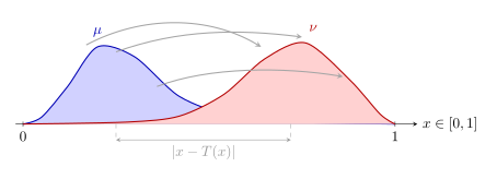
![Illustration of the Wasserstein distance for two distributions on $[0,1]$. The blue density $\mu$ is transported to the red density $\nu$; in one dimension, the optimal map $T$ moves quantiles monotonically and $W_2$ averages the squared lengths $|x-T(x)|^2$ with respect to $\mu$.](source/fig/generated/wasserstein-distance.svg){width=100%}
### The Metric Space $(\mathcal{P}_p(\mathcal{X}), W_p)$
The basic geometric properties of Wasserstein space are classical.
::: {#prp-metric-properties .proposition title="Basic metric properties of $\mathcal{W}_p(\mathcal{X})$"}
Let $(\mathcal{X}, d)$ be complete and separable.
1. **Metric property.** $W_p$ is a genuine finite metric on $\mathcal{P}_p(\mathcal{X})$, and $(\mathcal{P}_p(\mathcal{X}), W_p)$ is complete and separable [@Villani2009, Definition 6.4; @AmbrosioGigliSavare2008, Proposition 7.1.5].
2. **Topology of convergence.** Convergence in $W_p$ is equivalent to weak convergence together with convergence of the $p$th moments [@Villani2009, Definition 6.8 and Theorem 6.9; @AmbrosioGigliSavare2008, Proposition 7.1.5].
3. **Geodesic property.** When the ground space is a complete separable locally compact length space and $p > 1$, the Wasserstein space is geodesic [@Villani2009, Corollary 7.22].
4. **Compactness.** If $\mathcal{X}$ is compact, then $\mathcal{P}_p(\mathcal{X})$ is compact in $W_p$ [@AmbrosioGigliSavare2008, Proposition 7.1.5].
:::
::: {.callout-note title="Weak convergence and convergence of $p$-th moments" collapse="true"}
Point (2) above states that $W_p(\mu_n, \mu) \to 0$ is equivalent to the combination of two conditions. Understanding each is essential for working with Wasserstein distances.
**Weak convergence.** A sequence of probability measures $\{\mu_n\}$ on a metric space $\mathcal{X}$ converges **weakly** to $\mu$, denoted $\mu_n \rightharpoonup \mu$, if
$$
\int_{\mathcal{X}} f(x)\,d\mu_n(x) \;\longrightarrow\; \int_{\mathcal{X}} f(x)\,d\mu(x) \qquad \forall f \in C_b(\mathcal{X}),
$$
where $C_b(\mathcal{X})$ is the space of bounded continuous real-valued functions on $\mathcal{X}$. Equivalently, $\mu_n(A) \to \mu(A)$ for every Borel set $A$ whose boundary has $\mu$-measure zero (the **Portmanteau theorem**). Intuitively, weak convergence captures convergence of the "shape" or "mass distribution" of the measures — the probability assigned to every reasonable set stabilizes.
**Convergence of the $p$-th moments.** The $p$-th moment (about a reference point $x_0$) is
$$
M_p(\mu; x_0) = \int_{\mathcal{X}} d(x, x_0)^p\, d\mu(x).
$$
In the $W_p$ convergence criterion, once $\mu_n \rightharpoonup \mu$ is known, it is enough to verify
$$
M_p(\mu_n;x_0)\longrightarrow M_p(\mu;x_0)
$$
for one $x_0\in\mathcal X$; the same convergence then holds for every choice of reference point. Without weak convergence, convergence of the scalar moments about one reference point need not imply convergence about another. Combined with weak convergence, moment convergence prevents a vanishing amount of probability from carrying nonvanishing $p$-transport cost arbitrarily far away. This is stronger than ordinary tightness.
**Why both conditions are needed.** The two conditions control complementary aspects:
- **Weak convergence without moment convergence.** On $\mathbb R$, let
$$
\mu_n=\left(1-\frac1n\right)\delta_0+\frac1n\delta_{n^2}.
$$
Then $\mu_n\rightharpoonup\delta_0$: the mass sent to $n^2$ has probability only $1/n$, so it is invisible in the limit to every bounded continuous test function. However,
$$
M_p(\mu_n;0)=\frac1n(n^2)^p=n^{2p-1},
\qquad
W_p^p(\mu_n,\delta_0)=n^{2p-1}.
$$
Thus $W_p(\mu_n,\delta_0)\to\infty$ for every $p\ge1$. Notice that $\{\mu_n\}$ is nevertheless tight; tightness alone does not control the $p$-th moment in the tails.
- **Moment convergence without weak convergence.** On $\mathbb R$, let
$$
\mu_n=
\begin{cases}
\delta_1, & n\ \text{even},\\
\delta_{-1}, & n\ \text{odd}.
\end{cases}
$$
For every $p\ge1$,
$$
M_p(\mu_n;0)=1=M_p(\delta_1;0)
$$
for all $n$, so the $p$-th moments about $0$ converge. Nevertheless, $\mu_n$ does not converge weakly: its even and odd subsequences converge to the distinct measures $\delta_1$ and $\delta_{-1}$. Correspondingly, $W_p(\mu_n,\delta_1)$ alternates between $0$ and $2$ and therefore does not tend to zero.
Together, weak convergence and $p$-th moment convergence are exactly what is needed for the transport cost $\inf_\pi \int d(x, y)^p\, d\pi(x, y)$ between $\mu_n$ and $\mu$ to vanish [@Villani2009, Theorem 6.9; @AmbrosioGigliSavare2008, §7.1].
:::
## The Euclidean Case: Brenier's Theorem and Displacement Interpolation
We now specialize to the important case $\mathcal{X} = \mathbb{R}^d$ with the Euclidean distance. For $\mu_0, \mu_1 \in \mathcal{P}_2(\mathbb{R}^d)$,
$$
W_2^2(\mu_0, \mu_1) = \inf_{\pi \in \Pi(\mu_0, \mu_1)} \int_{\mathbb{R}^d \times \mathbb{R}^d} \|x - y\|_2^2 \, d\pi(x, y).
$$
::: {#thm-brenier .theorem title="Brenier's theorem (optimal maps)"}
If $\mu_0$ is absolutely continuous with respect to Lebesgue measure, then the optimal coupling is induced by a **transport map**: there exists a convex function $\varphi$ such that the optimal map is $T = \nabla\varphi$ and
$$
W_2^2(\mu_0, \mu_1) = \int_{\mathbb{R}^d} \|x - T(x)\|_2^2 \, d\mu_0(x).
$$
:::
The map $T$ pushes $\mu_0$ forward to $\mu_1$, i.e., $(T)_\#\mu_0 = \mu_1$, and it is the gradient of a convex potential -- a structure reminiscent of monotonicity in one dimension.
::: {.callout-note title="Push-Forward Measure" collapse="true"}
Given a measurable map $T: \mathcal{X} \to \mathcal{Y}$ and a probability measure $\mu$ on $\mathcal{X}$, the **push-forward** (or image measure) $T_\#\mu$ is the measure on $\mathcal{Y}$ defined by
$$
(T_\#\mu)(B) = \mu\bigl(T^{-1}(B)\bigr) \qquad \text{for all measurable } B \subseteq \mathcal{Y}.
$$
In probabilistic language: if $X \sim \mu$, then $T(X) \sim T_\#\mu$. The transport condition $(T)_\#\mu_0 = \mu_1$ means that applying $T$ to a random draw from $\mu_0$ yields a random draw from $\mu_1$ — the map **rearranges** the mass of $\mu_0$ into the shape of $\mu_1$.
:::
The corresponding **constant-speed geodesic** is the displacement interpolation introduced by @McCann1997:
::: {#def-displacement-interpolation .definition title="Displacement interpolation"}
Let $\mu_0, \mu_1 \in \mathcal{P}_2(\mathbb{R}^d)$ with $\mu_0$ absolutely continuous, and let $T$ be the optimal transport map from $\mu_0$ to $\mu_1$. The displacement interpolation geodesic is
$$
\mu_t = (T_t)_\# \mu_0, \qquad T_t = (1-t)\mathrm{id} + tT, \qquad 0 \le t \le 1.
$$
:::
Thus the geodesic moves mass along straight lines: each particle at position $x$ under $\mu_0$ moves linearly to $T(x)$ at speed determined by $t$.
## One-Dimensional Wasserstein Space
The one-dimensional case is considerably simpler and provides a powerful computational tool.
::: {#thm-quantile-representation .theorem title="Quantile representation of $W_2$ on $\mathbb{R}$"}
Let $\mu, \nu \in \mathcal{P}_2(\mathbb{R})$ with distribution functions $F_\mu, F_\nu$ and quantile functions $F_\mu^{-1}, F_\nu^{-1}$. Then
$$
W_2^2(\mu, \nu) = \int_0^1 \bigl|F_\mu^{-1}(u) - F_\nu^{-1}(u)\bigr|^2 \, du.
$$
If $\mu$ is atomless, the optimal map is the monotone rearrangement
$$
T = F_\nu^{-1} \circ F_\mu,
$$
and the geodesic between $\mu$ and $\nu$ is obtained by linear interpolation of quantiles:
$$
F_{\mu_t}^{-1}(u) = (1-t)F_\mu^{-1}(u) + tF_\nu^{-1}(u), \qquad 0 \le t \le 1.
$$
:::
Consequently, the quantile map $\mu \mapsto F_\mu^{-1}$ is an **isometric embedding** of $\mathcal{P}_2(\mathbb{R})$ into $L^2(0,1)$, and its image is the closed convex cone of square-integrable nondecreasing functions [@Villani2003; @PanaretosZemel2020; @PetersenMueller2016].
::: {.callout-tip title="Special properties of $\mathcal{W}_2(\mathbb{R})$"}
These features make one-dimensional Wasserstein space particularly tractable:
- Geodesics are **unique and explicit** -- just interpolate quantiles.
- The space is **flat**: isometric to a closed convex subset of a Hilbert space.
- **Wasserstein barycenters** are obtained by averaging quantile functions:
$$
F_{\bar\mu}^{-1}(u) = \sum_{j=1}^m \lambda_j F_{\mu_j}^{-1}(u), \qquad \lambda_j \ge 0,\; \sum_{j=1}^m \lambda_j = 1.
$$
- Many statistical procedures reduce to ordinary Hilbert-space constructions after the quantile transformation.
:::
## Application: Income Distribution Dynamics — A Distribution-as-Data Paradigm {#sec-income-application}
The previous lectures (Lectures 6–9) treated covariance matrices as data objects living in the SPD cone $\mathcal{S}_{++}^p$. Wasserstein geometry opens a complementary door: treating entire **probability distributions** as data objects. This perspective is particularly natural in economics, where the unit of analysis is often a distribution rather than a scalar summary.
### Why Distributions Instead of Summary Statistics?
Consider the problem of comparing economic inequality across countries or over time. The standard approach uses scalar summaries such as the Gini coefficient, the share of income going to the top 1%, or the poverty rate at a fixed threshold. Each of these collapses a full distribution into a single number — discarding information about where in the distribution changes occur.
Two countries can have identical Gini coefficients but vastly different income distributions: one might have a squeezed middle class with modest top-tail concentration, while another might have a hollowed-out middle with extreme polarization. Scalar summaries are blind to these distinctions; the Wasserstein distance between the full distributions captures them.
Moreover, the **optimal transport map** itself is of direct economic interest. The map $T = F_{\nu}^{-1} \circ F_{\mu}$ from a base-year income distribution $\mu$ to a later-year distribution $\nu$ is precisely the **growth-incidence curve**: it shows, for each percentile $u$ of the base-year distribution, the income at the same percentile in the later year. Economists routinely use growth-incidence curves to answer questions like "did the poor benefit more than the rich from economic growth?" The Wasserstein geometry provides the mathematical framework for treating these curves as geodesics in distribution space.
### The Data Structure
A typical cross-country income distribution dataset has the following structure:
- **Observations:** Country $c$ at year $t$
- **Data for each observation:** Either microdata (individual/household incomes) or, more commonly, a set of quantile shares (e.g., the World Bank PovcalNet data reporting the income share of each decile, plus the top 5% and top 1%)
- **Derived object:** An empirical distribution $\mu_{c,t} \in \mathcal{P}_2(\mathbb{R}_+)$, constructed from the quantile information
Thus each country-year becomes a single point in Wasserstein space $\mathcal{W}_2(\mathbb{R})$. The distance $W_2(\mu_{c,t}, \mu_{c',t'})$ measures the overall difference between two income distributions, accounting for shifts in location (mean income), scale (inequality), and shape (asymmetry, tail behavior) simultaneously.
### The Wasserstein Lens on Distributional Change
When comparing income distributions, the Wasserstein distance decomposes the total change into interpretable components. In one dimension, the quantile representation gives
$$
W_2^2(\mu, \nu) = \int_0^1 |Q_\mu(u) - Q_\nu(u)|^2 \, du.
$$
The optimal transport map $T(u) = Q_\nu(u)$ (plotted against $Q_\mu(u)$) is the **quantile-quantile (Q-Q) plot** familiar to statisticians, but reinterpreted through the lens of optimal transport: it is the unique monotone map that pushes $\mu$ forward to $\nu$ with minimal total squared displacement.
### Interactive Exploration: Income Distribution Comparison
The following demo simulates income distributions for two hypothetical country-years and computes their Wasserstein distance, optimal transport map, and displacement interpolation. The income distributions are modeled as mixtures of lognormal distributions — a standard parametric form that captures the characteristic right-skewness and Pareto-like upper tail of empirical income data.
**Visual guide:**
- **Density plots:** The two income distributions (blue = country A, red = country B) and the geodesic interpolation (purple dashed)
- **Q-Q / growth-incidence plot:** The optimal transport map $T = Q_B \circ F_A$, showing how each percentile of country A's income distribution maps to the corresponding percentile of country B's distribution. The 45° line is the identity — deviations from it represent distributional change.
- **Displacement interpolation:** Slide $t$ to see the geodesic path between the two distributions — the smoothest morphing of one income distribution into the other.
```{ojs}
//| label: fig-income-wasserstein
//| fig-cap: "Interactive: Wasserstein distance between income distributions"
inc_countryA_control = Inputs.select(
  ["Developed economy (low inequality)", "Emerging economy (moderate inequality)", "Developing economy (high inequality)"],
  {value: "Developed economy (low inequality)", label: "Country A — income profile"}
)
inc_countryB_control = Inputs.select(
  ["Developed economy (low inequality)", "Emerging economy (moderate inequality)", "Developing economy (high inequality)"],
  {value: "Developing economy (high inequality)", label: "Country B — income profile"}
)
inc_t_control = Inputs.range([0, 1], {step: 0.02, value: 0.5, label: "Geodesic parameter t"})
inc_countryA = Generators.input(inc_countryA_control)
inc_countryB = Generators.input(inc_countryB_control)
inc_t = Generators.input(inc_t_control)

inc_controls_view = html`
<style>
  .inc-slider-grid { display:flex; flex-wrap:wrap; gap:6px 20px; width:100%; margin:0 0 12px; font:0.85em system-ui,sans-serif; container-type:inline-size; }
  .inc-slider-grid > * { flex:1 1 calc((100% - 20px)/2); min-width:0; margin:0; }
  .inc-slider-grid input[type="number"] { width:7.5rem !important; }
  @container (max-width:480px) { .inc-slider-grid > * { flex-basis:100%; } }
</style>
<div class="inc-slider-grid">
  <div>${inc_countryA_control}</div>
  <div>${inc_countryB_control}</div>
  <div>${inc_t_control}</div>
</div>`

// ---- Income distribution parameters (lognormal mixtures) ----
// Each profile defined by: mean income, Gini-like spread, top-tail heaviness
// Using a mixture of two lognormals: main body + Pareto-like upper tail

function incomeProfile(label) {
  switch (label) {
    case "Developed economy (low inequality)":
      return {
        // Main body: concentrated around moderate income
        w1: 0.88, mu1: Math.log(38), sigma1: 0.45,
        // Upper tail: modest
        w2: 0.12, mu2: Math.log(95), sigma2: 0.55,
        label: "Developed"
      };
    case "Emerging economy (moderate inequality)":
      return {
        // Main body: lower average but wider spread
        w1: 0.82, mu1: Math.log(18), sigma1: 0.60,
        // Upper tail: more pronounced
        w2: 0.18, mu2: Math.log(70), sigma2: 0.70,
        label: "Emerging"
      };
    case "Developing economy (high inequality)":
      return {
        // Main body: low income, wide spread
        w1: 0.75, mu1: Math.log(8), sigma1: 0.70,
        // Upper tail: extreme concentration
        w2: 0.25, mu2: Math.log(55), sigma2: 0.85,
        label: "Developing"
      };
    default:
      return { w1: 1.0, mu1: Math.log(30), sigma1: 0.5, w2: 0.0, mu2: 0, sigma2: 0, label: "Default" };
  }
}

// ---- Quantile function from lognormal mixture ----
// CDF: F(x) = w1 * Phi((log x - mu1)/sigma1) + w2 * Phi((log x - mu2)/sigma2)
function makeIncomeQuantile(profile) {
  const {w1, mu1, sigma1, w2, mu2, sigma2} = profile;

  // Standard normal CDF
  function phi(z) { return 0.5 * (1 + erf(z / Math.sqrt(2))); }
  function erf(x) {
    const sign = x >= 0 ? 1 : -1;
    x = Math.abs(x);
    const a1 = 0.254829592, a2 = -0.284496736, a3 = 1.421413741;
    const a4 = -1.453152027, a5 = 1.061405429, p = 0.3275911;
    const t = 1 / (1 + p * x);
    const y = 1 - (((((a5 * t + a4) * t) + a3) * t + a2) * t + a1) * t * Math.exp(-x * x);
    return sign * y;
  }

  function mixCDF(x) {
    if (x <= 0) return 0;
    const z1 = (Math.log(x) - mu1) / sigma1;
    let f = w1 * phi(z1);
    if (w2 > 0) {
      const z2 = (Math.log(x) - mu2) / sigma2;
      f += w2 * phi(z2);
    }
    return f;
  }

  return function(u) {
    const uu = Math.max(1e-10, Math.min(1 - 1e-10, u));
    // Binary search for quantile
    let lo = 0.1, hi = 500;
    // Expand upper bound if needed
    while (mixCDF(hi) < uu && hi < 10000) hi *= 2;
    for (let k = 0; k < 60; k++) {
      const mid = (lo + hi) / 2;
      if (mixCDF(mid) < uu) lo = mid;
      else hi = mid;
    }
    return (lo + hi) / 2;
  };
}

// ---- Density function from profile ----
function makeIncomeDensity(profile) {
  const {w1, mu1, sigma1, w2, mu2, sigma2} = profile;
  return function(x) {
    if (x <= 0) return 0;
    let d = 0;
    const z1 = (Math.log(x) - mu1) / sigma1;
    d += (w1 / (x * sigma1 * Math.sqrt(2 * Math.PI))) * Math.exp(-0.5 * z1 * z1);
    if (w2 > 0) {
      const z2 = (Math.log(x) - mu2) / sigma2;
      d += (w2 / (x * sigma2 * Math.sqrt(2 * Math.PI))) * Math.exp(-0.5 * z2 * z2);
    }
    return d;
  };
}

// ---- Compute Wasserstein quantities ----
function computeIncomeDemo(profileA, profileB, t) {
  const QA = makeIncomeQuantile(profileA);
  const QB = makeIncomeQuantile(profileB);
  const densA = makeIncomeDensity(profileA);
  const densB = makeIncomeDensity(profileB);

  // Quantiles at a fine grid
  const nU = 300;
  const uGrid = Array.from({length: nU}, (_, i) => (i + 0.5) / nU);
  const qA = uGrid.map(u => QA(u));
  const qB = uGrid.map(u => QB(u));
  const qGeod = uGrid.map((u, i) => (1 - t) * qA[i] + t * qB[i]);

  // Geodesic quantile function
  const QGeod = u => (1 - t) * QA(u) + t * QB(u);

  // Density grid (log-spaced for better visualization)
  const nX = 250;
  const xMin = 0.1, xMax = 200;
  const xGrid = Array.from({length: nX}, (_, i) => xMin * Math.pow(xMax / xMin, i / (nX - 1)));

  const pdfA = xGrid.map(x => densA(x));
  const pdfB = xGrid.map(x => densB(x));

  // Geodesic density via derivative of quantile
  function densFromQuantile(Q, xGrid2) {
    const n2 = xGrid2.length;
    const cdf2 = xGrid2.map(x => {
      let lo = 0, hi = 1;
      for (let k = 0; k < 50; k++) {
        const mid = (lo + hi) / 2;
        if (Q(mid) < x) lo = mid;
        else hi = mid;
      }
      return (lo + hi) / 2;
    });
    const pdf2 = cdf2.map((_, i) => {
      if (i === 0) return Math.max(0, cdf2[1] / (xGrid2[1] - xGrid2[0]));
      if (i === n2 - 1) return Math.max(0, (1 - cdf2[n2 - 2]) / (xGrid2[n2 - 1] - xGrid2[n2 - 2]));
      return Math.max(0, (cdf2[i + 1] - cdf2[i - 1]) / (xGrid2[i + 1] - xGrid2[i - 1]));
    });
    return pdf2;
  }
  const pdfGeod = densFromQuantile(QGeod, xGrid);

  // Wasserstein distance
  let w2Sq = 0;
  for (let i = 0; i < nU; i++) {
    const d = qA[i] - qB[i];
    w2Sq += d * d / nU;
  }
  const w2 = Math.sqrt(w2Sq);

  // Mean incomes
  const meanA = qA.reduce((s, v) => s + v, 0) / nU;
  const meanB = qB.reduce((s, v) => s + v, 0) / nU;

  // Gini-like: relative mean absolute difference / (2 * mean)
  function giniFromQuantiles(q) {
    const n = q.length;
    let sumDiff = 0;
    for (let i = 0; i < n; i++) {
      for (let j = 0; j < n; j++) {
        sumDiff += Math.abs(q[i] - q[j]);
      }
    }
    const mean = q.reduce((s, v) => s + v, 0) / n;
    return sumDiff / (2 * n * n * mean);
  }
  const giniA = giniFromQuantiles(qA);
  const giniB = giniFromQuantiles(qB);

  // Transport map data for Q-Q plot
  const transportPts = Array.from({length: 100}, (_, i) => ({x: qA[Math.floor(i / 99 * (nU - 1))], y: qB[Math.floor(i / 99 * (nU - 1))]}));

  // Key percentiles for annotation
  const pctiles = {p10: 0.10, p50: 0.50, p90: 0.90, p99: 0.99};
  const keyPts = {};
  for (const [k, u] of Object.entries(pctiles)) {
    keyPts[k] = {qA: QA(u), qB: QB(u), u: u};
  }

  return {
    uGrid, qA, qB, qGeod,
    xGrid, pdfA, pdfB, pdfGeod,
    transportPts, keyPts,
    w2Sq, w2, meanA, meanB, giniA, giniB,
    t, profileA, profileB
  };
}

incResult = computeIncomeDemo(
  incomeProfile(inc_countryA),
  incomeProfile(inc_countryB),
  inc_t
);

// ---- Render income comparison visualization ----
html`
<div style="font-family: system-ui, sans-serif; max-width: 900px;">

  <h4>Income Distribution Comparison via Wasserstein Geometry</h4>

  <div style="display: flex; gap: 20px; flex-wrap: wrap;">

    <!-- Density Panel -->
    <div style="flex: 1; min-width: 420px;">
      <svg width="100%" height="240" viewBox="0 0 440 240" style="border: 1px solid #dee2e6; border-radius: 4px;">
        ${(() => {
          const margin = {top: 15, right: 15, bottom: 32, left: 50};
          const plotW = 440 - margin.left - margin.right;
          const plotH = 240 - margin.top - margin.bottom;

          const xGrid2 = incResult.xGrid, xMin2 = xGrid2[0], xMax2 = xGrid2[xGrid2.length - 1];
          const allPdf = [...incResult.pdfA, ...incResult.pdfB, ...incResult.pdfGeod];
          const yMax = Math.max(...allPdf) * 1.15;

          function xS(x) { return margin.left + Math.log(x / xMin2) / Math.log(xMax2 / xMin2) * plotW; }
          function yS(y) { return margin.top + plotH - (y / yMax) * plotH; }

          // Area fills
          function areaPath(pdf, color, opacity) {
            const pts = xGrid2.map((x, i) => `${xS(x)},${yS(pdf[i])}`).join(' ');
            return `<polygon points="${xS(xMin2)},${yS(0)} ${pts} ${xS(xMax2)},${yS(0)}" fill="${color}" fill-opacity="${opacity}" stroke="none"/>`;
          }
          function linePath(pdf, color, width, dash) {
            const pts = xGrid2.map((x, i) => `${i === 0 ? 'M' : 'L'} ${xS(x)} ${yS(pdf[i])}`).join(' ');
            return `<path d="${pts}" fill="none" stroke="${color}" stroke-width="${width}" stroke-dasharray="${dash || 'none'}"/>`;
          }

          // Tick marks at meaningful incomes
          const ticks = [0.5, 1, 2, 5, 10, 20, 50, 100, 200];

          const bg = `
            <line x1="${margin.left}" y1="${margin.top}" x2="${margin.left}" y2="${margin.top + plotH}" stroke="#adb5bd"/>
            <line x1="${margin.left}" y1="${margin.top + plotH}" x2="${margin.left + plotW}" y2="${margin.top + plotH}" stroke="#adb5bd"/>
            <text x="${margin.left - 5}" y="${margin.top - 3}" text-anchor="end" font-size="9" fill="#495057">density</text>
            <text x="${margin.left + plotW/2}" y="${margin.top + plotH + 20}" text-anchor="middle" font-size="10" fill="#495057">Income (thousands, log scale)</text>
            ${ticks.filter(t => t >= xMin2 && t <= xMax2).map(t => `<text x="${xS(t)}" y="${margin.top + plotH + 13}" text-anchor="middle" font-size="7.5" fill="#868e96">${t >= 1 ? '$' + t + 'k' : '$' + (t*1000)}</text>`).join('')}
            <text x="${margin.left + plotW/2}" y="${margin.top - 2}" text-anchor="middle" font-size="10" font-weight="bold" fill="#37474f">Income Densities and Geodesic Interpolation</text>
          `;

          const areas = `
            ${areaPath(incResult.pdfA, '#1971c2', 0.18)}
            ${areaPath(incResult.pdfB, '#e03131', 0.18)}
            ${areaPath(incResult.pdfGeod, '#7950f2', 0.10)}
          `;
          const lines = `
            ${linePath(incResult.pdfA, '#1971c2', 2.2)}
            ${linePath(incResult.pdfB, '#e03131', 2.2)}
            ${linePath(incResult.pdfGeod, '#6741d9', 2, '6,3')}
          `;

          // Mean income markers
          const meanMarkers = `
            <line x1="${xS(incResult.meanA)}" y1="${margin.top}" x2="${xS(incResult.meanA)}" y2="${margin.top + plotH}" stroke="#1971c2" stroke-width="1" stroke-dasharray="4,3" opacity="0.5"/>
            <text x="${xS(incResult.meanA) + 3}" y="${margin.top + 12}" font-size="8" fill="#1971c2">μ<sub>A</sub>=$${incResult.meanA.toFixed(1)}k</text>
            <line x1="${xS(incResult.meanB)}" y1="${margin.top}" x2="${xS(incResult.meanB)}" y2="${margin.top + plotH}" stroke="#e03131" stroke-width="1" stroke-dasharray="4,3" opacity="0.5"/>
            <text x="${xS(incResult.meanB) + 3}" y="${margin.top + 24}" font-size="8" fill="#e03131">μ<sub>B</sub>=$${incResult.meanB.toFixed(1)}k</text>
          `;

          return bg + areas + lines + meanMarkers + `<rect x="${margin.left}" y="${margin.top}" width="${plotW}" height="${plotH}" fill="none" stroke="#dee2e6"/>`;
        })()}
      </svg>

      <div style="display: flex; gap: 14px; justify-content: center; margin-top: 6px; font-size: 11px;">
        <span><span style="display:inline-block;width:16px;height:3px;background:#1971c2;"></span> ${incResult.profileA.label} (Gini ${incResult.giniA.toFixed(3)})</span>
        <span><span style="display:inline-block;width:16px;height:3px;background:#e03131;"></span> ${incResult.profileB.label} (Gini ${incResult.giniB.toFixed(3)})</span>
        <span><span style="display:inline-block;width:16px;height:3px;background:#6741d9;border-top:2px dashed #6741d9;"></span> μ<sub>t</sub> (t = ${incResult.t.toFixed(2)})</span>
      </div>
    </div>

    <!-- Q-Q / Growth-Incidence Panel -->
    <div style="flex: 1; min-width: 420px;">
      <svg width="100%" height="240" viewBox="0 0 440 240" style="border: 1px solid #dee2e6; border-radius: 4px;">
        ${(() => {
          const margin = {top: 15, right: 15, bottom: 32, left: 50};
          const plotW = 440 - margin.left - margin.right;
          const plotH = 240 - margin.top - margin.bottom;

          const allVals = [...incResult.transportPts.map(p => p.x), ...incResult.transportPts.map(p => p.y)];
          const qMin = Math.min(...allVals) * 0.9, qMax = Math.max(...allVals) * 1.1;

          function xS(x) { return margin.left + (x - qMin) / (qMax - qMin) * plotW; }
          function yS(y) { return margin.top + plotH - (y - qMin) / (qMax - qMin) * plotH; }

          // Identity line
          const diag = `M ${xS(qMin)} ${yS(qMin)} L ${xS(qMax)} ${yS(qMax)}`;

          // Transport map curve
          const mapPts = incResult.transportPts.map(p => `L ${xS(p.x)} ${yS(p.y)}`).join(' ');
          const mapPath = `M ${mapPts.substring(2)}`;

          // Key percentile annotations
          const keyAnnot = Object.entries(incResult.keyPts).map(([k, pt]) => {
            const label = k === 'p10' ? '10th' : k === 'p50' ? 'Median' : k === 'p90' ? '90th' : '99th';
            return `
              <circle cx="${xS(pt.qA)}" cy="${yS(pt.qB)}" r="4" fill="#7950f2" stroke="#fff" stroke-width="1.5"/>
              <text x="${xS(pt.qA) + 6}" y="${yS(pt.qB) + 3}" font-size="8" fill="#7950f2">${label}</text>
            `;
          }).join('');

          const bg = `
            <defs>
              <marker id="incArrow" markerWidth="6" markerHeight="4" refX="6" refY="2" orient="auto">
                <polygon points="0 0, 6 2, 0 4" fill="#adb5bd"/>
              </marker>
            </defs>
            <line x1="${margin.left}" y1="${margin.top}" x2="${margin.left}" y2="${margin.top + plotH}" stroke="#adb5bd"/>
            <line x1="${margin.left}" y1="${margin.top + plotH}" x2="${margin.left + plotW}" y2="${margin.top + plotH}" stroke="#adb5bd"/>
            <text x="${margin.left + plotW/2}" y="${margin.top + plotH + 20}" text-anchor="middle" font-size="10" fill="#495057">Income in A (thousands)</text>
            <text x="${margin.left - 42}" y="${margin.top + plotH/2}" text-anchor="middle" font-size="10" fill="#495057" transform="rotate(-90,${margin.left - 42},${margin.top + plotH/2})">Income in B (thousands)</text>
            <path d="${diag}" fill="none" stroke="#dee2e6" stroke-width="1.2" stroke-dasharray="4,4"/>
            <text x="${xS(qMax*0.85)}" y="${yS(qMax*0.78)}" font-size="8" fill="#adb5bd" font-style="italic">identity (no change)</text>
            <text x="${margin.left + plotW/2}" y="${margin.top - 2}" text-anchor="middle" font-size="10" font-weight="bold" fill="#37474f">Optimal Transport Map (Growth-Incidence Curve)</text>
          `;

          return bg + `<path d="${mapPath}" fill="none" stroke="#7950f2" stroke-width="2.5" stroke-linecap="round"/>` + keyAnnot + `<rect x="${margin.left}" y="${margin.top}" width="${plotW}" height="${plotH}" fill="none" stroke="#dee2e6"/>`;
        })()}
      </svg>
      <div style="text-align:center; margin-top:6px; font-size:11px; color:#495057;">
        <span style="display:inline-block;width:16px;height:3px;background:#7950f2;"></span> T = Q<sub>B</sub> ∘ F<sub>A</sub> — each percentile of A maps to the same percentile of B
      </div>
    </div>
  </div>

  <!-- Stats panel -->
  <div style="margin-top: 14px; padding: 12px; background: #f8f9fa; border-radius: 6px; display: flex; gap: 20px; flex-wrap: wrap;">
    <div style="flex: 1; min-width: 140px;">
      <b>W₂ distance:</b>
      <div style="font-size: 1.3em; font-weight: bold; color: #1971c2;">$${incResult.w2.toFixed(1)}k</div>
      <div style="font-size: 0.8em; color: #868e96;">W₂² = ${incResult.w2Sq.toFixed(1)} (thousands²)</div>
    </div>
    <div style="flex: 1; min-width: 140px;">
      <b>Mean shift:</b>
      <div style="font-size: 1.0em;">Δμ = $${(incResult.meanB - incResult.meanA).toFixed(1)}k</div>
      <div style="font-size: 0.8em; color: #868e96;">A: $${incResult.meanA.toFixed(1)}k → B: $${incResult.meanB.toFixed(1)}k</div>
    </div>
    <div style="flex: 1; min-width: 140px;">
      <b>Inequality (Gini):</b>
      <div style="font-size: 1.0em;">A: ${incResult.giniA.toFixed(3)} → B: ${incResult.giniB.toFixed(3)}</div>
      <div style="font-size: 0.8em; color: #868e96;">ΔGini = ${(incResult.giniB - incResult.giniA).toFixed(3)}</div>
    </div>
    <div style="flex: 1; min-width: 140px;">
      <b>Geodesic at t = ${incResult.t.toFixed(2)}:</b>
      <div style="font-size: 0.85em;">Q<sub>t</sub> = (1−t)Q<sub>A</sub> + tQ<sub>B</sub></div>
      <div style="font-size: 0.8em; color: #868e96;">Linear interpolation of quantile functions</div>
    </div>
  </div>

  <div style="margin-top: 12px; padding: 12px; background: #f1f3f5; border-radius: 6px; font-size: 0.9em;">
    <b>🔑 How to interpret the growth-incidence curve:</b>
    Points <b>above the diagonal</b> indicate that the corresponding percentile in country B earns <b>more</b> than the same percentile in country A.
    Points <b>below the diagonal</b> indicate the opposite.
    The further the curve deviates from the diagonal, the larger the distributional change at that income level.
    The W₂ distance aggregates these deviations (in the L² sense) into a single metric of overall distributional difference.
    <br><br>
    <b>📊 Preview — Wasserstein barycenters and regression:</b>
    With this distribution-as-data perspective, we can naturally ask:
    <ul style="margin: 4px 0 4px 16px;">
      <li><b>Barycenters:</b> What is the <i>average income distribution</i> of a group of countries? (Wasserstein barycenter = average of quantile functions)</li>
      <li><b>Regression:</b> How does a country's income distribution change with GDP growth, education, or trade openness? (Wasserstein regression with distribution-valued responses)</li>
      <li><b>Distributional counterfactuals:</b> What would country A's income distribution look like if it had country B's mean income but its own inequality structure? (Geodesic displacement interpolation)</li>
    </ul>
  </div>

</div>
`
```
::: {.callout-tip title="Try these experiments"}
- **Compare developed vs. developing:** The W₂ distance is large, reflecting differences in both mean income and inequality. The transport map lies substantially above the diagonal (B's rich are richer) but the lower percentiles may be below the diagonal.
- **Compare two developed economies** with the same profile: The W₂ distance should be zero — identical distributions.
- **Slide $t$ from 0 to 1:** Watch how the income distribution morphs from country A to country B. The geodesic shows the "smoothest" possible transition between the two distributions.
- **Note the growth-incidence curve shape:** If it crosses the diagonal, some percentiles in B are worse off than the same percentiles in A, even if B's mean is higher — a distributional pattern invisible to scalar comparisons.
- **Compare the Gini coefficients:** Even with similar Gini values, the W₂ distance can be large due to differences in mean income. This illustrates that W₂ captures both location and shape differences simultaneously.
:::
### From Distribution Comparison to Distributional Data Analysis
The income distribution example illustrates the core paradigm shift that Wasserstein geometry enables:
| Traditional approach | Distribution-as-data approach |
|---|---|
| Compare scalar summaries (mean, Gini, top-1% share) | Compare full distributions via $W_2$ |
| Ask "did inequality increase?" | Ask "how did the entire distribution shift, and at which percentiles?" |
| Regression of Gini on GDP | Regression of the full income distribution on GDP (Wasserstein regression) |
| Average Gini across countries | Wasserstein barycenter of income distributions (average of quantile functions) |
This paradigm will be developed systematically in the following lectures on Wasserstein barycenters and Wasserstein regression. The key computational advantage is that in one dimension, all operations reduce to working with quantile functions in $L^2(0,1)$ — a Hilbert space where averaging, linear regression, and ANOVA all have closed-form solutions.
## Alexandrov Curvature of Wasserstein Spaces
A geodesic metric space $(Y, d_Y)$ has **nonnegative Alexandrov curvature** (is a $\mathrm{CBB}(0)$ space) if for every constant-speed geodesic $\gamma: [0,1] \to Y$ from $y_0$ to $y_1$ and every $z \in Y$,
$$
d_Y^2(z, \gamma(t)) \ge (1-t) d_Y^2(z, y_0) + t d_Y^2(z, y_1) - t(1-t) d_Y^2(y_0, y_1),
\qquad 0 \le t \le 1.
$$
The opposite inequality characterizes **nonpositive curvature** ($\mathrm{CAT}(0)$).
::: {#thm-wasserstein-curvature .theorem title="Alexandrov curvature of Wasserstein spaces"}
1. **Inheritance of nonnegative curvature.** If the ground space $\mathcal{X}$ is a complete separable geodesic Alexandrov space with curvature bounded below by $0$, then $(\mathcal{W}_2(\mathcal{X}), W_2)$ also has Alexandrov curvature bounded below by $0$ [@Sturm2006GeometryI, Proposition 2.10].
2. **Compact Riemannian manifolds.** If $\mathcal{X}$ is a smooth compact connected Riemannian manifold, then $\mathcal{X}$ has nonnegative sectional curvature if and only if $(\mathcal{P}_2(\mathcal{X}), W_2)$ has nonnegative Alexandrov curvature [@LottVillani2009, Theorem A.8].
3. **The Euclidean line is flat.** Under the quantile isometry, $\mathcal{W}_2(\mathbb{R})$ is isometric to a closed convex cone of $L^2(0,1)$. Hence every Wasserstein triangle satisfies the Euclidean comparison identity [@Kloeckner2010, Proposition 4.1]:
$$
W_2^2(\nu, \mu_t) = (1-t)W_2^2(\nu, \mu_0) + tW_2^2(\nu, \mu_1) - t(1-t)W_2^2(\mu_0, \mu_1).
$$
4. **Higher dimensions are $\mathrm{CBB}(0)$ but not $\mathrm{CAT}(0)$.** Combining Sturm's theorem with the flat geometry of $\mathbb{R}^d$ gives
$$
(\mathcal{W}_2(\mathbb{R}^d), W_2) \in \mathrm{CBB}(0) \qquad \text{for every } d \ge 1.
$$
For $d = 1$ the space is flat. For $d \ge 2$, @Kloeckner2010 shows the flat identity fails: there exist pairs of Wasserstein geodesics with the same endpoints obtained from measures supported on orthogonal subspaces, so $\mathcal{W}_2(\mathbb{R}^d)$ is not $\mathrm{CAT}(0)$. Kloeckner describes this as positive sectional curvature at arbitrarily small scales. Thus $\mathcal{W}_2(\mathbb{R}^d)$ for $d \ge 2$ is a canonical example of a space with an Alexandrov lower curvature bound of $0$ but no matching upper bound.
:::
## Computation of Wasserstein Distances and Optimal Transport
While the theoretical formulation of the Wasserstein distance is elegant, practical computation requires careful algorithmic choices. The computational landscape splits naturally into three regimes: the **general discrete case** (linear programming), the **one-dimensional case** (monotone matching), and **entropy-regularized approximations** (Sinkhorn algorithm).
### General Discrete Formulation: The Kantorovich Linear Program
Let $\mu = \sum_{i=1}^n a_i \delta_{x_i}$ and $\nu = \sum_{j=1}^m b_j \delta_{y_j}$ be discrete probability measures with weight vectors $\mathbf{a} \in \Delta_n$, $\mathbf{b} \in \Delta_m$ (the probability simplices) and support points $x_i, y_j \in \mathbb{R}^d$. The $p$-Wasserstein distance is the solution to the **Kantorovich optimal transport problem**:
$$
W_p^p(\mu, \nu) = \min_{P \in \mathbb{R}_+^{n \times m}} \sum_{i=1}^n \sum_{j=1}^m C_{ij} P_{ij}
$$
subject to the marginal constraints
$$
\sum_{j=1}^m P_{ij} = a_i \quad (i = 1, \ldots, n), \qquad
\sum_{i=1}^n P_{ij} = b_j \quad (j = 1, \ldots, m),
$$
where $C_{ij} = \|x_i - y_j\|^p$ is the ground cost matrix. The decision variable $P = (P_{ij})$ is the **transport plan** (coupling matrix); $P_{ij}$ is the amount of mass transported from $x_i$ to $y_j$.
This is a **linear program** (LP) with $nm$ nonnegative variables and $n+m$ marginal equalities. One equality is redundant because both measures have total mass one, leaving $n+m-1$ independent equalities. A dense formulation requires at least $O(nm)$ input and storage just for the cost matrix. There is no algorithm-independent $O((nm)^3)$ complexity bound: classical simplex pivot rules can take exponentially many pivots in the worst case, while polynomial interior-point bounds depend on the particular formulation, solver, and linear-algebra structure. General-purpose solvers also return an unregularized optimum only up to their numerical feasibility and optimality tolerances.
::: {.callout-note title="Network flow perspective"}
The Kantorovich problem is a minimum-cost flow problem on a complete bipartite graph with $V=n+m$ vertices and $E=nm$ edges. Network-simplex and transportation-simplex methods exploit this structure and are often fast in practice, but there is no universal $O(n^3\log n)$ bound: worst-case behavior depends on the pivot rule, and classical rules can require exponentially many pivots.
These algorithms accept an arbitrary finite cost matrix $C$; metric costs are not required by the solver. If $C_{ij}=d(x_i,y_j)^p$, the optimum is $W_p^p$. For a general $C$, it is an optimal **transport cost**, but it need not induce a Wasserstein distance or any metric.
:::
### One-Dimensional Case: Monotone Matching
When $d = 1$, the problem collapses to a beautifully simple computation. For empirical measures with $n$ points each and equal weights $a_i = b_j = 1/n$, the optimal transport plan is the **order-preserving (monotone) matching**: sort the points of both measures and match the $k$-th smallest element of $\mu$ to the $k$-th smallest element of $\nu$.
::: {#alg-sort-match .algorithm title="1D Wasserstein Distance — Monotone Matching"}
**Input:** Vectors $\mathbf{x} = (x_1, \ldots, x_n)$, $\mathbf{y} = (y_1, \ldots, y_m)$, weights $\mathbf{a} \in \Delta_n$, $\mathbf{b} \in \Delta_m$.
**Step 1:** Sort $\mathbf{x}$ in ascending order: $x_{(1)} \le x_{(2)} \le \cdots \le x_{(n)}$.
**Step 2:** Sort $\mathbf{y}$ in ascending order: $y_{(1)} \le y_{(2)} \le \cdots \le y_{(m)}$.
**Step 3 (equal weights, $n = m$):** The optimal transport plan is the diagonal matching $P_{(i)(i)} = 1/n$, and
$$
W_2^2(\mu, \nu) = \frac{1}{n}\sum_{i=1}^n |x_{(i)} - y_{(i)}|^2.
$$
**Step 3 (general weights or unequal support sizes):** Sweep through the sorted supports and their cumulative masses. At the current pair $(i,j)$, transport the smaller of the two remaining masses, subtract it from both remainders, and advance every index whose remainder reaches zero. This produces the exact monotone coupling and is equivalent to integrating the two empirical quantile functions.
**Complexity:** Sorting costs $O(n\log n+m\log m)$ and the cumulative-mass sweep costs $O(n+m)$. If both supports are already sorted, the complete computation is $O(n+m)$.
:::
The proof is a direct consequence of the quantile representation (@thm-quantile-representation): the map $\mu \mapsto F_\mu^{-1}$ is an isometry into $L^2(0,1)$, and empirical quantile functions are obtained from sorted supports and cumulative weights. Simple index-by-index matching is valid only for equal weights and equal support sizes; the weighted sweep is needed in general.
::: {.callout-important title="Why 1D is special"}
The sort-and-match algorithm exploits the total order on $\mathbb{R}$. In higher dimensions, there is no canonical ordering, and the optimal transport plan can be genuinely two-dimensional (mass splits across multiple destinations). This fundamental difference explains why $\mathcal{W}_2(\mathbb{R}^d)$ for $d \ge 2$ is computationally harder and geometrically more curved than the flat $\mathcal{W}_2(\mathbb{R})$.
:::
### Entropic Regularization and the Sinkhorn Algorithm
The breakthrough that made large-scale optimal transport feasible came from **entropic regularization** [@CuturiDoucet2014]. Add an entropy penalty to the LP objective:
$$
\min_{P \in \Pi(\mathbf{a}, \mathbf{b})} \sum_{i=1}^n \sum_{j=1}^m C_{ij} P_{ij} - \varepsilon H(P),
$$
where $H(P)=-\sum_{ij}P_{ij}(\log P_{ij}-1)$ is an entropy functional (the Shannon entropy plus a constant on probability couplings), and $\varepsilon>0$ is the regularization strength. The regularized objective is strictly convex on the positive entries, so it selects a unique plan after zero-mass rows and columns are removed.
::: {#thm-sinkhorn-structure .theorem title="Structure of the entropic optimal transport plan"}
The unique minimizer $P^\varepsilon$ of the entropy-regularized problem has the form
$$
P_{ij}^\varepsilon = u_i K_{ij} v_j, \qquad K_{ij} = \exp\!\left(-\frac{C_{ij}}{\varepsilon}\right),
$$
where $\mathbf{u} \in \mathbb{R}_+^n$, $\mathbf{v} \in \mathbb{R}_+^m$ are positive scaling vectors determined by the marginal constraints $\sum_j P_{ij}^\varepsilon = a_i$ and $\sum_i P_{ij}^\varepsilon = b_j$. The matrix $K = (K_{ij})$ is the **Gibbs kernel** — a pairwise similarity matrix derived from the cost via exponentiation.
:::
The structure $P^\varepsilon = \operatorname{diag}(\mathbf{u}) K \operatorname{diag}(\mathbf{v})$ reduces the problem from optimizing over $nm$ variables to finding $n + m$ scaling parameters. The **Sinkhorn–Knopp algorithm** (also known as iterative proportional fitting) solves for $\mathbf{u}$ and $\mathbf{v}$ by alternating row and column normalizations:
::: {#alg-sinkhorn .algorithm title="Sinkhorn–Knopp Algorithm for Entropic Optimal Transport"}
**Input:** Cost matrix $C$, weight vectors $\mathbf{a}, \mathbf{b}$, regularization $\varepsilon > 0$, tolerance $\delta > 0$.
**Step 1:** Form the Gibbs kernel $K_{ij} = \exp(-C_{ij} / \varepsilon)$.
**Step 2:** Initialize $\mathbf{v}^{(0)} = \mathbf{1}_m$ (or $\mathbf{v}^{(0)} = \mathbf{b}$).
**Step 3:** For $t = 0, 1, 2, \ldots$ until convergence:
$$
u_i^{(t+1)} = \frac{a_i}{\sum_{j} K_{ij} v_j^{(t)}} \quad (i = 1, \ldots, n),
\qquad
v_j^{(t+1)} = \frac{b_j}{\sum_{i} K_{ij} u_i^{(t+1)}} \quad (j = 1, \ldots, m).
$$
**Step 4:** Stop when $\|P\mathbf{1}_m - \mathbf{a}\|_1 + \|P^\top\mathbf{1}_n - \mathbf{b}\|_1 < \delta$, where $P_{ij} = u_i K_{ij} v_j$.
**Output:** The entropy-regularized transport plan $P^\varepsilon$. Its raw transport cost $\sum_{ij}C_{ij}P_{ij}^\varepsilon$ and its regularized objective value are distinct quantities.
:::
Each dense Sinkhorn iteration costs $O(nm)$, so $T$ iterations cost $O(Tnm)$ arithmetic operations. Storing a dense cost matrix or Gibbs kernel costs $O(nm)$ memory; explicitly constructing pairwise costs for points in $\mathbb{R}^d$ can additionally require $O(nmd)$ work. The iteration count $T$ is not fixed: it depends on $\varepsilon$, the scale and dynamic range of $C$, the requested marginal and objective accuracy, the stopping rule, and the numerical stabilization and rounding procedures.
::: {.callout-note title="Convergence properties"}
For a strictly positive Gibbs kernel, Sinkhorn iterations converge to the unique entropy-regularized optimum (after zero-mass rows and columns are removed). Geometric convergence can be stated in a projective metric, but its constants deteriorate when $\varepsilon$ is small relative to the range of the costs. Ordinary-domain iterations can then underflow, and log-domain stabilization is often needed.
On a fixed finite problem, as $\varepsilon\to0$, $P^\varepsilon$ converges to the maximum-entropy member of the set of unregularized optimal plans; the unregularized optimum need not be unique. As $\varepsilon\to\infty$, $P^\varepsilon$ converges to the independent coupling $P_{ij}=a_ib_j$.
For finite supports, an objective-value bias bound is controlled by $\varepsilon$ times an entropy range and can contain a worst-case factor of order $\log(nm)$. This is not a bound on the transport plan. Regularization bias, marginal residual, and floating-point error are separate quantities and should be assessed separately.
:::
### Comparison of Algorithms
| Method | Computational cost | Best for | Main limitations |
|---|---:|---|---|
| **General-purpose LP** | Classical simplex pivot rules have exponential worst-case examples; interior-point complexity depends on the formulation and solver [@KleeMinty1972; @NesterovNemirovskii1994]. | Small problems, arbitrary costs and constraints, and an unregularized optimum | At least $O(nm)$ dense input/storage [@PeyreCuturi2019, sec. 3.1]; generic solvers do not exploit the transport-network structure; solutions satisfy numerical tolerances rather than symbolic exactness |
| **Network simplex / transportation simplex** | The graph has $V=n+m$ and $E=nm$; worst-case pivot counts depend on the rule and can be exponential [@Cunningham1979; @AhujaOrlin1992]. | Small-to-medium unregularized discrete OT, arbitrary finite costs, and sparse optimal plans | Dense problems require storing or accessing $nm$ costs [@PeyreCuturi2019, secs. 3.1 and 3.5]; degeneracy and the pivot rule can strongly affect runtime |
| **1D monotone matching** | $O(n\log n+m\log m)$ to sort, followed by an $O(n+m)$ cumulative-mass sweep; $O(n+m)$ if already sorted [@PeyreCuturi2019, sec. 2.6]. | Exact $W_p$ and an exact monotone coupling on $\mathbb{R}$ for $p\ge1$ | Applies directly only in one dimension; pairwise rank matching requires equal weights and equal support sizes |
| **Sinkhorn** | $O(Tnm)$ for $T$ dense iterations and $O(nm)$ naive memory; constructing all pairwise costs may cost $O(nmd)$ [@PeyreCuturi2019, sec. 4.2]. | Differentiable, GPU-friendly entropy-regularized OT for moderate dense problems; larger problems with convolutional, sparse, low-rank, or matrix-free structure | Produces a generally dense regularized plan; bias depends on $\varepsilon$, support size, entropy convention, and problem structure; small $\varepsilon$ worsens convergence and stability |
| **Sinkhorn with $\varepsilon$-scaling / annealing** | $O\!\left(nm\sum_k T_k\right)$ for a dense schedule, with $T_k$ iterations at level $\varepsilon_k$ [@Schmitzer2019, secs. 3.2 and 4.4]. | Warm-starting computations at small regularization and obtaining more accurate entropy-regularized OT | A schedule alone does not guarantee a near-exact unregularized solution; total work depends on the schedule and stopping criteria; the final small-$\varepsilon$ problem remains ill-conditioned |
The practical choice depends on structure and required accuracy: use the monotone cumulative-mass sweep in one dimension; use an unregularized transport solver when that optimum is required and the problem is manageable; use Sinkhorn for entropy-regularized OT, especially when the kernel can be applied without materializing a dense matrix. A naive dense kernel with $n=m=10^5$ has $10^{10}$ entries—about $40$ GB in single precision for the kernel alone—so a GPU by itself does not make that case practical.
### Interactive Exploration: Discrete Optimal Transport and the Sinkhorn Algorithm
The following demo illustrates the Sinkhorn algorithm on two discrete distributions in 1D. You can adjust the positions and weights of the points, the regularization strength $\varepsilon$, and step through iterations to see the transport plan converge.
**Visual guide:**
- **Top panel:** The two point masses on the real line, with the transport plan shown as arrows (thickness ∝ mass transported).
- **Bottom left:** The coupling matrix $P_{ij}$ as a heatmap — each cell shows the amount of mass transported from $x_i$ to $y_j$.
- **Bottom right:** Convergence diagnostics — marginal error and transport cost vs. iteration.
```{ojs}
//| output: false
sk_n_control = Inputs.range([4, 12], {step: 1, value: 6, label: "Number of points per distribution"})
sk_eps_control = Inputs.range([0.001, 3], {step: 0.001, value: 0.6, label: "Entropy ε"})
sk_iter_control = Inputs.range([0, 200], {step: 1, value: 40, label: "Sinkhorn iterations"})
sk_seed_control = Inputs.range([1, 50], {step: 1, value: 7, label: "Random seed"})
sk_n = Generators.input(sk_n_control)
sk_eps = Generators.input(sk_eps_control)
sk_iter = Generators.input(sk_iter_control)
sk_seed = Generators.input(sk_seed_control)

sk_controls_view = html`
<style>
  .sk-slider-grid { display:grid; grid-template-columns:repeat(2,minmax(0,1fr)); gap:6px 20px; max-width:620px; margin:0 auto 12px; font:0.85em system-ui,sans-serif; }
  .sk-slider-grid > * { min-width:0; margin:0; }
  .sk-slider-grid input[type="number"] { width:7.5rem !important; }
  @media (max-width:500px) { .sk-slider-grid { grid-template-columns:1fr; } }
</style>
<div class="sk-slider-grid">
  <div>${sk_n_control}</div>
  <div>${sk_eps_control}</div>
  <div>${sk_iter_control}</div>
  <div>${sk_seed_control}</div>
</div>`

function otSvgFragment(markup) {
  const wrapper = document.createElementNS("http://www.w3.org/2000/svg", "svg");
  wrapper.innerHTML = markup;
  const fragment = document.createDocumentFragment();
  while (wrapper.firstChild) fragment.appendChild(wrapper.firstChild);
  return fragment;
}

// ---- Sinkhorn Algorithm Implementation ----

function sinkhornDemo(n, epsilon, maxIter, seed) {
  // Seeded RNG
  let s = seed;
  function rng() {
    s |= 0; s = s + 0x6D2B79F5 | 0;
    let t = Math.imul(s ^ s >>> 15, 1 | s);
    t = t + Math.imul(t ^ t >>> 7, 61 | t) ^ t;
    return ((t ^ t >>> 14) >>> 0) / 4294967296;
  }

  // Generate two sets of points (1D, overlapping ranges)
  const xPts = Array.from({length: n}, (_, i) => -2 + rng() * 5 + (i / n) * 3);
  const yPts = Array.from({length: n}, (_, i) => -2 + rng() * 5 + (i / n) * 2.5);
  xPts.sort((a, b) => a - b);
  yPts.sort((a, b) => a - b);

  // Equal weights
  const a = Array.from({length: n}, () => 1 / n);
  const b = Array.from({length: n}, () => 1 / n);

  // Cost matrix: squared Euclidean distance
  const C = Array.from({length: n}, (_, i) =>
    Array.from({length: n}, (_, j) => {
      const d = xPts[i] - yPts[j];
      return d * d;
    })
  );

  // Gibbs kernel
  const K = C.map(row => row.map(c => Math.exp(-c / Math.max(epsilon, 1e-12))));

  // Sinkhorn iterations
  let u = Array(n).fill(1);
  let v = Array(n).fill(1);
  const history = [];

  // Initial P (no iterations yet)
  const P0 = Array.from({length: n}, (_, i) =>
    Array.from({length: n}, (_, j) => u[i] * K[i][j] * v[j])
  );
  const rowSum0 = P0.map(row => row.reduce((s, val) => s + val, 0));
  const colSum0 = Array.from({length: n}, (_, j) =>
    P0.reduce((s, row) => s + row[j], 0)
  );
  const margErr0 = rowSum0.reduce((s, r, i) => s + Math.abs(r - a[i]), 0) +
    colSum0.reduce((s, c, j) => s + Math.abs(c - b[j]), 0);
  const cost0 = P0.reduce((s, row, i) =>
    s + row.reduce((si, p, j) => si + C[i][j] * p, 0), 0
  );
  history.push({iter: 0, margErr: margErr0, cost: cost0, u: [...u], v: [...v]});

  for (let t = 1; t <= maxIter; t++) {
    // Update u
    for (let i = 0; i < n; i++) {
      let sum = 0;
      for (let j = 0; j < n; j++) sum += K[i][j] * v[j];
      u[i] = a[i] / Math.max(sum, 1e-16);
    }
    // Update v
    for (let j = 0; j < n; j++) {
      let sum = 0;
      for (let i = 0; i < n; i++) sum += K[i][j] * u[i];
      v[j] = b[j] / Math.max(sum, 1e-16);
    }

    // Compute current P and diagnostics
    if (t % Math.max(1, Math.floor(maxIter / 50)) === 0 || t === maxIter) {
      const P = Array.from({length: n}, (_, i) =>
        Array.from({length: n}, (_, j) => u[i] * K[i][j] * v[j])
      );
      const rowSum = P.map(row => row.reduce((s, val) => s + val, 0));
      const colSum = Array.from({length: n}, (_, j) =>
        P.reduce((s, row) => s + row[j], 0)
      );
      const margErr = rowSum.reduce((s, r, i) => s + Math.abs(r - a[i]), 0) +
        colSum.reduce((s, c, j) => s + Math.abs(c - b[j]), 0);
      const cost = P.reduce((s, row, i) =>
        s + row.reduce((si, p, j) => si + C[i][j] * p, 0), 0
      );
      history.push({iter: t, margErr, cost, u: [...u], v: [...v]});
    }
  }

  // Compute final P
  const Pfinal = Array.from({length: n}, (_, i) =>
    Array.from({length: n}, (_, j) => u[i] * K[i][j] * v[j])
  );

  // Ground truth (1D optimal: sort-and-match)
  const xSorted = [...xPts].sort((a, b) => a - b);
  const ySorted = [...yPts].sort((a, b) => a - b);
  let w2exactSq = 0;
  for (let i = 0; i < n; i++) {
    const d = xSorted[i] - ySorted[i];
    w2exactSq += d * d / n;
  }
  const w2exact = Math.sqrt(w2exactSq);

  // Current cost
  const finalCost = Pfinal.reduce((s, row, i) =>
    s + row.reduce((si, p, j) => si + C[i][j] * p, 0), 0
  );

  // Currently displayed iteration (from slider)
  const displayIter = Math.min(maxIter, sk_iter);
  // Find closest history entry
  let bestHist = history[0];
  for (const h of history) {
    if (h.iter <= displayIter) bestHist = h;
  }

  // Compute P at the displayed iteration
  const uDisp = bestHist.u;
  const vDisp = bestHist.v;
  const Pdisp = Array.from({length: n}, (_, i) =>
    Array.from({length: n}, (_, j) => uDisp[i] * K[i][j] * vDisp[j])
  );

  return {
    n, epsilon, maxIter,
    xPts, yPts, a, b, C, K,
    Pfinal, finalCost,
    Pdisp, displayIter,
    history,
    w2exact, w2exactSq,
    bestHist
  };
}

skResult = sinkhornDemo(sk_n, sk_eps, sk_iter, sk_seed);

// ---- Render Sinkhorn visualization ----
function renderSkDemo(skResult, sk_controls_view) {
return html`
<div style="font-family: system-ui, sans-serif; max-width: 920px;">

  <h4>Discrete Optimal Transport — Sinkhorn Algorithm in Action</h4>
  ${sk_controls_view}

  <!-- Panel 1: Points on line with transport arrows -->
  <div style="margin-bottom: 14px;">
    <svg width="100%" height="190" viewBox="0 0 900 190" style="border: 1px solid #dee2e6; border-radius: 4px;">
      ${(() => {
        const margin = {top: 35, right: 30, bottom: 30, left: 20};
        const plotW = 900 - margin.left - margin.right;
        const plotH = 190 - margin.top - margin.bottom;

        const allVals = [...skResult.xPts, ...skResult.yPts];
        const xMin = Math.min(...allVals) - 0.5;
        const xMax = Math.max(...allVals) + 0.5;

        function xS(x) { return margin.left + (x - xMin) / (xMax - xMin) * plotW; }

        // Thickness scaling for transport arrows
        const P = skResult.Pdisp;
        const maxP = Math.max(...P.flat());
        const n = skResult.n;

        // Source and target y-positions — all points on one horizontal line each
        const srcY = margin.top + plotH * 0.18;
        const tgtY = margin.top + plotH * 0.82;

        // Build transport arrows (only show significant ones)
        let arrows = '';
        const threshold = maxP * 0.03;
        for (let i = 0; i < n; i++) {
          for (let j = 0; j < n; j++) {
            if (P[i][j] > threshold) {
              const xi = xS(skResult.xPts[i]);
              const xj = xS(skResult.yPts[j]);
              const yi = srcY;
              const yj = tgtY;
              const alpha = Math.min(1, P[i][j] / maxP);
              const width = Math.max(0.5, 4 * P[i][j] / maxP);
              // Curved path
              const midX = (xi + xj) / 2;
              const cpX = midX + (j - i) * 6;
              arrows += `<path d="M ${xi} ${yi} Q ${cpX} ${(yi + yj)/2} ${xj} ${yj}" fill="none" stroke="#7950f2" stroke-width="${width.toFixed(1)}" opacity="${alpha.toFixed(2)}" stroke-linecap="round"/>`;
            }
          }
        }

        // Point markers — all source points on srcY, all target points on tgtY
        let sourcePts = '';
        for (let i = 0; i < n; i++) {
          const sx = xS(skResult.xPts[i]);
          const labY = i % 2 === 0 ? srcY - 9 : srcY - 19;
          sourcePts += `<circle cx="${sx}" cy="${srcY}" r="5.5" fill="#1971c2" stroke="#fff" stroke-width="1.5"/>`;
          sourcePts += `<text x="${sx}" y="${labY}" text-anchor="middle" font-size="8.5" fill="#1971c2">x<tspan baseline-shift="sub" font-size="6.5">${i+1}</tspan></text>`;
        }
        let targetPts = '';
        for (let j = 0; j < n; j++) {
          const tx = xS(skResult.yPts[j]);
          const labY = j % 2 === 0 ? tgtY + 15 : tgtY + 25;
          targetPts += `<circle cx="${tx}" cy="${tgtY}" r="5.5" fill="#e03131" stroke="#fff" stroke-width="1.5"/>`;
          targetPts += `<text x="${tx}" y="${labY}" text-anchor="middle" font-size="8.5" fill="#e03131">y<tspan baseline-shift="sub" font-size="6.5">${j+1}</tspan></text>`;
        }

        // X-axis tick values
        const tickVals = [];
        for (let v = Math.ceil(xMin); v <= Math.floor(xMax); v++) tickVals.push(v);

        return otSvgFragment(`
          <text x="${margin.left + plotW/2}" y="16" text-anchor="middle" font-size="11" font-weight="bold" fill="#37474f">Transport Plan: Arrows show mass flow from source μ (top) to target ν (bottom)</text>
          <text x="${margin.left + plotW/2}" y="32" text-anchor="middle" font-size="9" fill="#868e96">Arrow thickness ∝ mass transported. Only flows above 3% of max are shown.</text>
          <line x1="${margin.left}" y1="${margin.top + plotH}" x2="${margin.left + plotW}" y2="${margin.top + plotH}" stroke="#adb5bd"/>
          ${tickVals.map(v => `<line x1="${xS(v)}" y1="${margin.top + plotH}" x2="${xS(v)}" y2="${margin.top + plotH + 4}" stroke="#adb5bd"/><text x="${xS(v)}" y="${margin.top + plotH + 14}" text-anchor="middle" font-size="8" fill="#868e96">${v}</text>`).join("")}
          ${arrows}
          ${sourcePts}
          ${targetPts}
          <text x="${margin.left + plotW/2}" y="${margin.top + plotH + 18}" text-anchor="middle" font-size="10" fill="#495057">Position (1D)</text>
          <rect x="${margin.left}" y="${margin.top}" width="${plotW}" height="${plotH}" fill="none" stroke="#dee2e6"/>
          <g transform="translate(${margin.left + plotW + 10}, ${margin.top + 4})">
            <circle cx="6" cy="0" r="5" fill="#1971c2" stroke="#fff" stroke-width="1.2"/><text x="14" y="4" font-size="9" fill="#495057">Source μ</text>
            <circle cx="6" cy="18" r="5" fill="#e03131" stroke="#fff" stroke-width="1.2"/><text x="14" y="22" font-size="9" fill="#495057">Target ν</text>
          </g>
        `);
      })()}
    </svg>
  </div>

  <div style="display: flex; gap: 16px; flex-wrap: wrap;">

    <!-- Coupling Matrix Heatmap -->
    <div style="flex: 1; min-width: 380px;">
      <svg width="100%" height="260" viewBox="0 0 420 260" style="border: 1px solid #dee2e6; border-radius: 4px;">
        ${(() => {
          const margin = {top: 30, right: 10, bottom: 35, left: 40};
          const size = 260 - margin.top - margin.bottom;
          const n = skResult.n;
          const cellW = size / n, cellH = size / n;
          const P = skResult.Pdisp;
          const maxP = Math.max(...P.flat());

          // Color scale: light gray → medium purple → dark purple
          function color(p) {
            const t = maxP > 1e-12 ? p / maxP : 0;
            // Interpolate from light gray (#e9ecef) to dark purple (#4a1a8a)
            const r = Math.round(233 - t * 158);
            const g = Math.round(236 - t * 216);
            const b2 = Math.round(239 - t * 101);
            return `rgb(${r},${g},${b2})`;
          }

          let cells = '';
          for (let i = 0; i < n; i++) {
            for (let j = 0; j < n; j++) {
              const x = margin.left + j * cellW;
              const y = margin.top + i * cellH;
              cells += `<rect x="${x}" y="${y}" width="${cellW}" height="${cellH}" fill="${color(P[i][j])}" stroke="#ced4da" stroke-width="0.8"/>`;
              if (P[i][j] > maxP * 0.15) {
                cells += `<text x="${x + cellW/2}" y="${y + cellH/2 + 3}" text-anchor="middle" font-size="${Math.max(7, 10 - n)}" fill="${P[i][j] > maxP * 0.5 ? '#fff' : '#495057'}">${(P[i][j] * 100).toFixed(0)}</text>`;
              }
            }
          }

          return otSvgFragment(`
            <text x="${margin.left + size/2}" y="14" text-anchor="middle" font-size="10" font-weight="bold" fill="#37474f">Coupling Matrix P<tspan baseline-shift="sub" font-size="7">ij</tspan> (heatmap)</text>
            ${cells}
            <text x="${margin.left + size/2}" y="${margin.top + size + 20}" text-anchor="middle" font-size="10" fill="#495057">y<tspan baseline-shift="sub" font-size="7">j</tspan> (target)</text>
            <text x="${margin.left - 32}" y="${margin.top + size/2}" text-anchor="middle" font-size="10" fill="#495057" transform="rotate(-90,${margin.left - 32},${margin.top + size/2})">x<tspan baseline-shift="sub" font-size="7">i</tspan> (source)</text>
            <!-- Color bar -->
            ${(() => {
              let bar = '';
              for (let k = 0; k < 10; k++) {
                const t = k / 9;
                const y = margin.top + 5 + k * 10;
                const r2 = Math.round(233 - t * 158);
                const g2 = Math.round(236 - t * 216);
                const b3 = Math.round(239 - t * 101);
                bar += `<rect x="${margin.left + size + 8}" y="${y}" width="10" height="10" fill="rgb(${r2},${g2},${b3})" stroke="none"/>`;
              }
              bar += `<text x="${margin.left + size + 22}" y="${margin.top + 10}" font-size="7" fill="#495057">${(maxP * 100).toFixed(1)}%</text>`;
              bar += `<text x="${margin.left + size + 22}" y="${margin.top + 5 + 9 * 10 + 4}" font-size="7" fill="#495057">0%</text>`;
              return bar;
            })()}
            <rect x="${margin.left}" y="${margin.top}" width="${size}" height="${size}" fill="none" stroke="#dee2e6"/>
          `);
        })()}
      </svg>
      <div style="text-align:center; margin-top:4px; font-size:10px; color:#868e96;">
        Each cell P<sub>ij</sub>: mass from x<sub>i</sub> → y<sub>j</sub>. Darker = more mass.
      </div>
    </div>

    <!-- Convergence Plot -->
    <div style="flex: 1; min-width: 380px;">
      <svg width="100%" height="260" viewBox="0 0 420 260" style="border: 1px solid #dee2e6; border-radius: 4px;">
        ${(() => {
          const margin = {top: 30, right: 50, bottom: 32, left: 50};
          const plotW = 420 - margin.left - margin.right;
          const plotH = 260 - margin.top - margin.bottom;

          const hist = skResult.history;
          const maxIter = skResult.maxIter;

          const errMax = Math.max(...hist.map(h => h.margErr), 1e-10);
          const costMin = Math.min(...hist.map(h => h.cost), skResult.w2exactSq, 0);
          const costMax = Math.max(...hist.map(h => h.cost), skResult.w2exactSq, 1);

          function xS(t) { return margin.left + (maxIter > 0 ? t / maxIter : 0) * plotW; }

          // Left axis: marginal error
          function ySErr(e) { return margin.top + plotH - (e / errMax) * plotH * 0.9; }
          // Right axis: cost
          function ySCost(c) { return margin.top + plotH - ((c - costMin) / (costMax - costMin + 1e-10)) * plotH * 0.9; }

          // Error curve
          let errPath = '';
          hist.forEach((h, idx) => {
            errPath += `${idx === 0 ? 'M' : 'L'} ${xS(h.iter)} ${ySErr(h.margErr)}`;
          });

          // Cost curve
          let costPath = '';
          hist.forEach((h, idx) => {
            costPath += `${idx === 0 ? 'M' : 'L'} ${xS(h.iter)} ${ySCost(h.cost)}`;
          });

          // Exact W2 reference line
          const exactY = ySCost(skResult.w2exactSq);

          const bg = `
            <line x1="${margin.left}" y1="${margin.top}" x2="${margin.left}" y2="${margin.top + plotH}" stroke="#adb5bd"/>
            <line x1="${margin.left}" y1="${margin.top + plotH}" x2="${margin.left + plotW}" y2="${margin.top + plotH}" stroke="#adb5bd"/>
            <text x="${margin.left + plotW/2}" y="14" text-anchor="middle" font-size="10" font-weight="bold" fill="#37474f">Convergence Diagnostics</text>
            <text x="${margin.left + plotW/2}" y="${margin.top + plotH + 18}" text-anchor="middle" font-size="9" fill="#495057">Sinkhorn iteration</text>
          `;

          // Legend
          const legend = `
            <line x1="${margin.left + plotW - 170}" y1="${margin.top + 4}" x2="${margin.left + plotW - 155}" y2="${margin.top + 4}" stroke="#1971c2" stroke-width="2"/>
            <text x="${margin.left + plotW - 152}" y="${margin.top + 8}" font-size="8" fill="#495057">Marginal error (L)</text>
            <line x1="${margin.left + plotW - 170}" y1="${margin.top + 16}" x2="${margin.left + plotW - 155}" y2="${margin.top + 16}" stroke="#e03131" stroke-width="2"/>
            <text x="${margin.left + plotW - 152}" y="${margin.top + 20}" font-size="8" fill="#495057">Transport cost (R)</text>
            <line x1="${margin.left + plotW - 170}" y1="${margin.top + 28}" x2="${margin.left + plotW - 155}" y2="${margin.top + 28}" stroke="#2e7d32" stroke-width="1.5" stroke-dasharray="3,2"/>
            <text x="${margin.left + plotW - 152}" y="${margin.top + 32}" font-size="8" fill="#2e7d32">W₂² (exact 1D)</text>
          `;

          return otSvgFragment(bg + `
            <path d="${errPath}" fill="none" stroke="#1971c2" stroke-width="2" stroke-linecap="round"/>
            <path d="${costPath}" fill="none" stroke="#e03131" stroke-width="2" stroke-linecap="round"/>
            <line x1="${margin.left}" y1="${exactY}" x2="${margin.left + plotW}" y2="${exactY}" stroke="#2e7d32" stroke-width="1.5" stroke-dasharray="3,2"/>
            ${legend}
            <rect x="${margin.left}" y="${margin.top}" width="${plotW}" height="${plotH}" fill="none" stroke="#dee2e6"/>
          `);
        })()}
      </svg>
    </div>
  </div>

  <!-- Stats panel -->
  <div style="margin-top: 12px; padding: 12px; background: #f8f9fa; border-radius: 6px; font-size: 0.88em;">
    <table style="width:100%; border-collapse:collapse;">
      <tr style="border-bottom:1px solid #dee2e6;">
        <td style="padding:5px 8px;" colspan="3"><b>Sinkhorn Diagnostics</b> — ε = ${skResult.epsilon.toFixed(3)}, n = ${skResult.n}, iteration ${skResult.bestHist.iter} / ${skResult.maxIter}</td>
      </tr>
      <tr>
        <td style="padding:4px 8px;">Current plan cost</td>
        <td style="padding:4px 8px; text-align:right; font-family:monospace; color:#e03131;">${skResult.finalCost.toFixed(4)}</td>
        <td style="padding:4px 8px; font-size:0.85em; color:#868e96;">Raw transport cost; compare only when marginal error is small</td>
      </tr>
      <tr>
        <td style="padding:4px 8px;">Exact W₂² (1D sort)</td>
        <td style="padding:4px 8px; text-align:right; font-family:monospace; color:#2e7d32; font-weight:bold;">${skResult.w2exactSq.toFixed(4)}</td>
        <td style="padding:4px 8px; font-size:0.85em; color:#868e96;">Ground truth: sort-and-match</td>
      </tr>
      <tr>
        <td style="padding:4px 8px;">Raw cost gap</td>
        <td style="padding:4px 8px; text-align:right; font-family:monospace; ${skResult.finalCost < skResult.w2exactSq ? 'color:#e03131;' : ''}">${(skResult.finalCost - skResult.w2exactSq).toFixed(4)}</td>
        <td style="padding:4px 8px; font-size:0.85em; color:#868e96;">Nonnegative for a converged feasible plan; not a bias estimate while infeasible</td>
      </tr>
      <tr>
        <td style="padding:4px 8px;">Marginal error L₁</td>
        <td style="padding:4px 8px; text-align:right; font-family:monospace;">${skResult.bestHist.margErr.toExponential(3)}</td>
        <td style="padding:4px 8px; font-size:0.85em; color:#868e96;">Constraint violation (→ 0 at convergence)</td>
      </tr>
      <tr style="border-top:1px solid #dee2e6;">
        <td style="padding:4px 8px;" colspan="3">
          <b>${skResult.bestHist.margErr < 0.01 ?
            '✅ Near-convergence — marginal error < 0.01.' :
            skResult.bestHist.margErr < 0.1 ?
            '⏳ Moderate convergence — run more iterations for tighter marginals.' :
            '🔴 Far from convergence — increase iterations or increase ε for faster convergence.'}
          </b>
          ${skResult.epsilon < 0.01 ? ' Note: Very small ε can require many iterations and may need log-domain stabilization.' : ''}
          ${skResult.epsilon > 1.5 ? ' Note: Large ε produces a blurry (high-entropy) plan. Reduce ε for a sharper plan closer to the true optimal transport.' : ''}
        </td>
      </tr>
    </table>
  </div>

</div>
`
}
```
```{ojs}
//| label: fig-sinkhorn-demo
//| fig-cap: "Interactive: Sinkhorn algorithm for discrete optimal transport"
renderSkDemo(skResult, sk_controls_view)
```
::: {.callout-tip title="Try these experiments"}
- **Set ε large ($\varepsilon \ge 1.5$):** The Sinkhorn algorithm converges in very few iterations, but the transport plan is diffuse (mass spreads across many targets). The coupling matrix shows a blurry band rather than a sharp diagonal.
- **Set ε small ($\varepsilon \le 0.05$):** The transport plan sharpens toward the true optimal matching (nearly diagonal in 1D), but convergence slows dramatically — watch the marginal error decay slowly.
- **Increase iterations from 0 to 200:** Watch the marginal error decrease as the matrix scalings enforce feasibility. Intermediate raw costs need not be monotone or comparable with $W_2^2$ because the intermediate matrix may violate the marginals.
- **Compare with the exact 1D solution:** The green dashed line shows the unregularized $W_2^2$ from monotone matching. Once the Sinkhorn plan is feasible, its raw transport cost is at least this optimum; for a fixed finite problem, the gap vanishes as $\varepsilon\to0$ when the regularized problems are solved accurately.
- **Change the random seed:** Different point configurations produce different transport patterns. Try seeds that create overlapping vs. separated clusters.
:::
### Interactive Exploration: 1D Sort-and-Match Algorithm
This simpler demo illustrates the **sort-and-match algorithm** on empirical distributions. Since the optimal transport in 1D is order-preserving, sorting both sets of points and matching by rank gives the exact solution — no iteration needed.
```{ojs}
//| output: false
sm_n_control = Inputs.range([4, 20], {step: 1, value: 8, label: "Number of points n"})
sm_seed2_control = Inputs.range([1, 50], {step: 1, value: 13, label: "Random seed"})
sm_n = Generators.input(sm_n_control)
sm_seed2 = Generators.input(sm_seed2_control)

sm_controls_view = html`
<style>
  .sm-slider-grid { display:grid; grid-template-columns:repeat(2,minmax(0,1fr)); gap:6px 20px; max-width:620px; margin:0 auto 12px; font:0.85em system-ui,sans-serif; }
  .sm-slider-grid > * { min-width:0; margin:0; }
  .sm-slider-grid input[type="number"] { width:7.5rem !important; }
  @media (max-width:500px) { .sm-slider-grid { grid-template-columns:1fr; } }
</style>
<div class="sm-slider-grid">
  <div>${sm_n_control}</div>
  <div>${sm_seed2_control}</div>
</div>`

function sortMatchDemo(n, seed) {
  let s = seed;
  function rng() {
    s |= 0; s = s + 0x6D2B79F5 | 0;
    let t = Math.imul(s ^ s >>> 15, 1 | s);
    t = t + Math.imul(t ^ t >>> 7, 61 | t) ^ t;
    return ((t ^ t >>> 14) >>> 0) / 4294967296;
  }

  // Two sets of points with different distributions
  const xRaw = Array.from({length: n}, () => -1 + rng() * 6);
  const yRaw = Array.from({length: n}, () => 0 + rng() * 5);

  // Sort for optimal matching
  const xSorted = [...xRaw].sort((a, b) => a - b);
  const ySorted = [...yRaw].sort((a, b) => a - b);

  // Compute W2 distance
  let w2Sq = 0;
  const matches = [];
  for (let i = 0; i < n; i++) {
    const d = xSorted[i] - ySorted[i];
    w2Sq += d * d / n;
    matches.push({x: xSorted[i], y: ySorted[i], d});
  }
  const w2 = Math.sqrt(w2Sq);

  // Naive (wrong) matching: match by index without sorting (to show contrast)
  let naiveW2Sq = 0;
  for (let i = 0; i < n; i++) {
    const d = xRaw[i] - yRaw[i];
    naiveW2Sq += d * d / n;
  }
  const naiveW2 = Math.sqrt(naiveW2Sq);

  // Cost matrix
  const C = xSorted.map(xi => ySorted.map(yj => {
    const d = xi - yj;
    return d * d;
  }));

  return {
    n, xRaw, yRaw, xSorted, ySorted,
    matches, w2Sq, w2, naiveW2Sq, naiveW2,
    C
  };
}

smResult = sortMatchDemo(sm_n, sm_seed2);

function renderSmDemo(smResult, sm_controls_view) {
return html`
<div style="font-family: system-ui, sans-serif; width: 100%;">
  <h4>1D Optimal Transport — Sort-and-Match Algorithm</h4>
  ${sm_controls_view}

  <div style="display: flex; flex-direction: column; align-items: center; gap: 16px; width: 100%;">

    <!-- Points on line with optimal matching -->
    <div style="width: 70%; max-width: 800px; margin-inline: auto;">
      <svg width="100%" height="280" viewBox="0 0 480 280" style="border: 1px solid #dee2e6; border-radius: 4px;">
        ${(() => {
          const margin = {top: 35, right: 20, bottom: 35, left: 50};
          const plotW = 480 - margin.left - margin.right;
          const plotH = 280 - margin.top - margin.bottom;

          const allVals = [...smResult.xSorted, ...smResult.ySorted];
          const xMin = Math.min(...allVals) - 0.5;
          const xMax = Math.max(...allVals) + 0.5;

          function xS(x) { return margin.left + (x - xMin) / (xMax - xMin) * plotW; }

          const n = smResult.n;

          // Sorted matching arrows with distance labels
          let arrows = '';
          smResult.matches.forEach((m, i) => {
            const xi = xS(m.x), yi = xS(m.y);
            const yTop = margin.top + 6 + i * (plotH - 86) / (n - 1);
            const yBot = yTop + 55;
            arrows += `<line x1="${xi}" y1="${yTop}" x2="${yi}" y2="${yBot}" stroke="#2e7d32" stroke-width="2.5" stroke-linecap="round" opacity="0.85"/>`;
            if (Math.abs(m.d) > 0.3) {
              arrows += `<text x="${(xi + yi)/2 + 4}" y="${(yTop + yBot)/2 + 4}" font-size="8" fill="#2e7d32" font-weight="bold">Δ${i+1}</text>`;
            }
            // Rank labels
            arrows += `<text x="${xi - 14}" y="${yTop + 4}" font-size="9" fill="#1971c2" text-anchor="end">x<tspan baseline-shift="sub" font-size="6.5">(${i+1})</tspan></text>`;
            arrows += `<text x="${yi - 14}" y="${yBot + 4}" font-size="9" fill="#e03131" text-anchor="end">y<tspan baseline-shift="sub" font-size="6.5">(${i+1})</tspan></text>`;
          });

          // Point markers
          let pts = '';
          smResult.xSorted.forEach((x, i) => {
            pts += `<circle cx="${xS(x)}" cy="${margin.top + 6 + i * (plotH - 86) / (n - 1)}" r="5.5" fill="#1971c2" stroke="#fff" stroke-width="2"/>`;
          });
          smResult.ySorted.forEach((y, i) => {
            pts += `<circle cx="${xS(y)}" cy="${margin.top + 61 + i * (plotH - 86) / (n - 1)}" r="5.5" fill="#e03131" stroke="#fff" stroke-width="2"/>`;
          });

          return otSvgFragment(`
            <text x="${margin.left + plotW/2}" y="14" text-anchor="middle" font-size="11" font-weight="bold" fill="#37474f">Optimal 1D Matching: Sort, Then Match by Rank</text>
            <text x="${margin.left + plotW/2}" y="28" text-anchor="middle" font-size="9" fill="#868e96">x<tspan baseline-shift="sub" font-size="6.5">(k)</tspan> ↔ y<tspan baseline-shift="sub" font-size="6.5">(k)</tspan>: the k-th smallest of μ matches the k-th smallest of ν</text>
            ${arrows}
            ${pts}
            <text x="${margin.left + plotW/2}" y="${margin.top + plotH + 20}" text-anchor="middle" font-size="10" fill="#495057">Position (1D)</text>
            <rect x="${margin.left}" y="${margin.top}" width="${plotW}" height="${plotH}" fill="none" stroke="#dee2e6"/>
            <g transform="translate(${margin.left + plotW + 5}, ${margin.top + 10})">
              <circle cx="6" cy="0" r="5" fill="#1971c2" stroke="#fff" stroke-width="1.5"/><text x="14" y="4" font-size="9" fill="#495057">Source μ</text>
              <circle cx="6" cy="18" r="5" fill="#e03131" stroke="#fff" stroke-width="1.5"/><text x="14" y="22" font-size="9" fill="#495057">Target ν</text>
            </g>
          `);
        })()}
      </svg>
    </div>

    <!-- Explanation panel -->
    <div style="width: 70%; max-width: 800px; margin-inline: auto;">
      <div style="padding: 14px; background: #f8f9fa; border-radius: 6px; font-size: 0.9em;">
        <b>Algorithm: Sort-and-Match</b>
        <ol style="margin: 8px 0 8px 16px; padding: 0;">
          <li>Sort ${smResult.n} source points: <var>x</var><sub>(1)</sub> ≤ ⋯ ≤ <var>x</var><sub>(${smResult.n})</sub></li>
          <li>Sort ${smResult.n} target points: <var>y</var><sub>(1)</sub> ≤ ⋯ ≤ <var>y</var><sub>(${smResult.n})</sub></li>
          <li>Match by rank: <var>x</var><sub>(k)</sub> ↔ <var>y</var><sub>(k)</sub></li>
          <li>W<sub>2</sub><sup>2</sup> = average of |<var>x</var><sub>(k)</sub> − <var>y</var><sub>(k)</sub>|<sup>2</sup></li>
        </ol>

        <table style="width:100%; margin-top:10px; border-collapse:collapse;">
          <tr><td style="padding:4px 8px;">W₂² (sort-and-match)</td>
              <td style="text-align:right; font-family:monospace; color:#2e7d32; font-weight:bold;">${smResult.w2Sq.toFixed(3)}</td></tr>
          <tr><td style="padding:4px 8px;">W₂</td>
              <td style="text-align:right; font-family:monospace; font-weight:bold;">${smResult.w2.toFixed(3)}</td></tr>
          <tr><td style="padding:4px 8px;">Naive (unsorted) W₂²</td>
              <td style="text-align:right; font-family:monospace; color:#e03131;">${smResult.naiveW2Sq.toFixed(3)}</td></tr>
          <tr style="border-top:1px solid #dee2e6;"><td style="padding:4px 8px;">Reduction</td>
              <td style="text-align:right; font-family:monospace; color:#2e7d38;">${((1 - smResult.w2Sq / smResult.naiveW2Sq) * 100).toFixed(0)}% lower cost</td></tr>
        </table>

        <div style="margin-top:12px; padding:8px; background:#e8f5e9; border-radius:4px; font-size:0.85em;">
          <b>✅ Optimality guarantee:</b> The sort-and-match solution is <i>globally optimal</i> — no other transport plan can achieve a lower total cost. This is a consequence of the quantile representation theorem.
        </div>
      </div>
    </div>
  </div>

</div>
`
}
```
```{ojs}
//| label: fig-sort-match
//| fig-cap: "Interactive: 1D sort-and-match for exact Wasserstein computation"
renderSmDemo(smResult, sm_controls_view)
```
::: {.callout-tip title="Key takeaway — why sorting works"}
The sort-and-match algorithm exploits the **total order** on $\mathbb{R}$. For the convex cost $|x-y|^p$, $p\ge1$, uncrossing oppositely ordered assignments cannot increase total cost; equivalently, the quantile coupling is optimal. Pairwise rank matching implements this argument for equally weighted samples, while a cumulative-mass sweep implements it for arbitrary discrete weights.
This gives an $O(n\log n+m\log m)$ algorithm for unsorted one-dimensional supports and an $O(n+m)$ algorithm for sorted supports. Higher dimensions have no analogous total order, so this reduction does not apply.
:::
### Practical Recommendations
1. **For one-dimensional data:** Use monotone matching. Match ranks only for equal weights and equal support sizes; otherwise use the cumulative-mass sweep. This computes the unregularized $W_p$ exactly up to floating-point arithmetic.
2. **When an unregularized optimum is required:** Use a network/transportation solver that exploits the bipartite structure, or a general LP when extra linear constraints are important. Feasible scale depends on density, memory, degeneracy, solver implementation, and accuracy requirements—not a universal sample-size cutoff.
3. **For differentiable entropy-regularized OT:** Use Sinkhorn. Dense implementations cost $O(Tnm)$ time and $O(nm)$ memory; genuinely large problems need convolutional, sparse, low-rank, blockwise, or matrix-free kernel operations.
4. **For small final regularization:** An $\varepsilon$-scaling schedule can warm-start successive problems, usually with log-domain stabilization. The schedule improves computation but does not itself certify a near-exact unregularized solution; check marginal residual, regularization bias, numerical error, and any final feasibility-rounding error separately.
## Interactive Exploration: Wasserstein Distance on $[0,1]$
The following demo visualizes the $W_2$ distance between two distributions on $[0,1]$ using the quantile representation. Adjust the shapes and see the optimal transport map, the displacement interpolation geodesic, and the computed distance.
```{ojs}
//| output: false
dist1_type_control = Inputs.select(
  ["gaussian", "uniform", "bimodal", "skewed"],
  {value: "gaussian", label: "Distribution 1 type"}
)
dist1_mean_control = Inputs.range([0.2, 0.8], {step: 0.05, value: 0.35, label: "Distribution 1 mean"})
dist1_spread_control = Inputs.range([0.05, 0.25], {step: 0.01, value: 0.12, label: "Distribution 1 spread"})

dist2_type_control = Inputs.select(
  ["gaussian", "uniform", "bimodal", "skewed"],
  {value: "bimodal", label: "Distribution 2 type"}
)
dist2_mean_control = Inputs.range([0.2, 0.8], {step: 0.05, value: 0.65, label: "Distribution 2 mean"})
dist2_spread_control = Inputs.range([0.05, 0.25], {step: 0.01, value: 0.10, label: "Distribution 2 spread"})

geodesic_t_control = Inputs.range([0, 1], {step: 0.02, value: 0.5, label: "Geodesic parameter t"})
dist1_type = Generators.input(dist1_type_control)
dist1_mean = Generators.input(dist1_mean_control)
dist1_spread = Generators.input(dist1_spread_control)
dist2_type = Generators.input(dist2_type_control)
dist2_mean = Generators.input(dist2_mean_control)
dist2_spread = Generators.input(dist2_spread_control)
geodesic_t = Generators.input(geodesic_t_control)

wasser_controls_view = html`
<style>
  .wasser-slider-grid { display:flex; flex-wrap:wrap; gap:6px 20px; width:100%; margin:0 0 12px; font:0.85em system-ui,sans-serif; container-type:inline-size; }
  .wasser-slider-grid > * { flex:1 1 calc((100% - 40px)/3); min-width:0; margin:0; }
  .wasser-slider-grid input[type="number"] { width:7.5rem !important; }
  @container (max-width:700px) { .wasser-slider-grid > * { flex-basis:calc((100% - 20px)/2); } }
  @container (max-width:480px) { .wasser-slider-grid > * { flex-basis:100%; } }
</style>
<div class="wasser-slider-grid">
  <div>${dist1_type_control}</div>
  <div>${dist1_mean_control}</div>
  <div>${dist1_spread_control}</div>
  <div>${dist2_type_control}</div>
  <div>${dist2_mean_control}</div>
  <div>${dist2_spread_control}</div>
  <div>${geodesic_t_control}</div>
</div>`

// Build distribution functions and compute Wasserstein quantities
function makeQuantileFn(type, mean, spread) {
  // Returns a quantile function Q(u) for u in [0,1]
  return function(u) {
    // Clamp for safety
    const uu = Math.max(1e-10, Math.min(1 - 1e-10, u));
    switch (type) {
      case "gaussian": {
        // Truncated Gaussian via inverse error function
        // Quantile of N(mean, spread^2), truncated to [0,1]
        const z = Math.sqrt(2) * erfinv(2 * uu - 1);
        const raw = mean + spread * z;
        return Math.max(0, Math.min(1, raw));
      }
      case "uniform": {
        const half = spread * Math.sqrt(3); // std dev -> half-width for uniform
        const lo = Math.max(0, mean - half);
        const hi = Math.min(1, mean + half);
        return lo + uu * (hi - lo);
      }
      case "bimodal": {
        // Mixture of two Gaussians: modes at mean +/- spread
        const m1 = Math.max(0.05, mean - spread * 0.8);
        const m2 = Math.min(0.95, mean + spread * 0.8);
        const s = spread * 0.5;
        // Inverse CDF via binary search on mixture CDF
        function mixCDF(x) {
          const z1 = (x - m1) / s;
          const z2 = (x - m2) / s;
          return 0.5 * (0.5 * (1 + erf(z1 / Math.sqrt(2))) + 0.5 * (1 + erf(z2 / Math.sqrt(2))));
        }
        // Binary search for quantile
        let lo = Math.max(0, Math.min(m1, m2) - 4 * s);
        let hi = Math.min(1, Math.max(m1, m2) + 4 * s);
        for (let i = 0; i < 50; i++) {
          const mid = (lo + hi) / 2;
          if (mixCDF(mid) < uu) lo = mid;
          else hi = mid;
        }
        return (lo + hi) / 2;
      }
      case "skewed": {
        // Beta distribution as a flexible skewed distribution
        // Map mean and spread to alpha, beta parameters
        const mu = Math.max(0.05, Math.min(0.95, mean));
        const v = spread * spread;
        const alpha = mu * (mu * (1 - mu) / v - 1);
        const beta = (1 - mu) * (mu * (1 - mu) / v - 1);
        const aa = Math.max(0.5, alpha);
        const bb = Math.max(0.5, beta);
        return betainv(uu, aa, bb);
      }
      default:
        return uu;
    }
  };
}

// Helper: inverse error function
function erfinv(x) {
  const a = 0.147;
  const ln1mx2 = Math.log(1 - x * x);
  const t = 2 / (Math.PI * a) + ln1mx2 / 2;
  const sqrtTerm = Math.sqrt(t * t - ln1mx2 / a);
  const y = Math.sqrt(sqrtTerm - t);
  return x >= 0 ? y : -y;
}

// Helper: error function
function erf(x) {
  const sign = x >= 0 ? 1 : -1;
  x = Math.abs(x);
  const a1 = 0.254829592, a2 = -0.284496736, a3 = 1.421413741;
  const a4 = -1.453152027, a5 = 1.061405429, p = 0.3275911;
  const t = 1 / (1 + p * x);
  const y = 1 - (((((a5 * t + a4) * t) + a3) * t + a2) * t + a1) * t * Math.exp(-x * x);
  return sign * y;
}

// Helper: regularized incomplete beta function (continued fraction)
function betainv(p, a, b) {
  if (p <= 0) return 0;
  if (p >= 1) return 1;
  // Binary search on regularized incomplete beta
  function betainc(x, aa, bb) {
    if (x <= 0 || x >= 1) return x <= 0 ? 0 : 1;
    // Use continued fraction representation
    const bt = Math.exp(lgamma(aa+bb) - lgamma(aa) - lgamma(bb) + aa*Math.log(x) + bb*Math.log(1-x));
    if (x < (aa+1)/(aa+bb+2)) {
      return bt * betacf(x, aa, bb) / aa;
    } else {
      return 1 - bt * betacf(1-x, bb, aa) / bb;
    }
  }
  function betacf(x, aa, bb) {
    const maxIter = 100;
    const eps = 3e-16;
    let qab = aa + bb;
    let qap = aa + 1;
    let qam = aa - 1;
    let c = 1;
    let d = 1 - qab * x / qap;
    if (Math.abs(d) < eps) d = eps;
    d = 1 / d;
    let result = d;
    for (let m = 1; m <= maxIter; m++) {
      const m2 = 2 * m;
      // Even step
      let aa_m = m * (bb - m) * x / ((qam + m2) * (aa + m2));
      d = 1 + aa_m * d;
      if (Math.abs(d) < eps) d = eps;
      c = 1 + aa_m / c;
      if (Math.abs(c) < eps) c = eps;
      d = 1 / d;
      result *= d * c;
      // Odd step
      aa_m = -(aa + m) * (qab + m) * x / ((aa + m2) * (qap + m2));
      d = 1 + aa_m * d;
      if (Math.abs(d) < eps) d = eps;
      c = 1 + aa_m / c;
      if (Math.abs(c) < eps) c = eps;
      d = 1 / d;
      const delta = d * c;
      result *= delta;
      if (Math.abs(delta - 1) < eps) break;
    }
    return result;
  }
  let lo = 0, hi = 1;
  for (let i = 0; i < 50; i++) {
    const mid = (lo + hi) / 2;
    const val = betainc(mid, a, b);
    if (val < p) lo = mid;
    else hi = mid;
  }
  return (lo + hi) / 2;
}

function lgamma(z) {
  // Stirling's approximation for log-gamma
  if (z < 0.5) {
    return Math.log(Math.PI / Math.sin(Math.PI * z)) - lgamma(1 - z);
  }
  z -= 1;
  const g = 7;
  const c = [0.99999999999980993, 676.5203681218851, -1259.1392167224028,
             771.32342877765313, -176.61502916214059, 12.507343278686905,
             -0.13857109526572012, 9.9843695780195716e-6, 1.5056327351493116e-7];
  let x = c[0];
  for (let i = 1; i < g + 2; i++) x += c[i] / (z + i);
  const t = z + g + 0.5;
  return 0.5 * Math.log(2 * Math.PI) + (z + 0.5) * Math.log(t) - t + Math.log(x);
}

// Compute densities from quantile functions
function densityFromQuantile(Q, xGrid) {
  // Approximate density via derivative of quantile inverse
  const n = xGrid.length;
  const dx = xGrid[1] - xGrid[0];
  const cdf = xGrid.map(x => {
    // Binary search: find u such that Q(u) = x
    let lo = 0, hi = 1;
    for (let i = 0; i < 40; i++) {
      const mid = (lo + hi) / 2;
      if (Q(mid) < x) lo = mid;
      else hi = mid;
    }
    return (lo + hi) / 2;
  });
  const pdf = cdf.map((_, i) => {
    // Use one-sided derivatives at the displayed boundaries. Do not force
    // F(0) = 0 or F(1) = 1: clamped quantiles can carry boundary atoms, and
    // folding those atoms into the first/last density bin creates spikes.
    if (i === 0) return (cdf[1] - cdf[0]) / dx;
    if (i === n-1) return (cdf[n-1] - cdf[n-2]) / dx;
    return (cdf[i+1] - cdf[i-1]) / (2 * dx);
  });
  return pdf.map(v => Math.max(0, v));
}

// Compute everything
function computeWassersteinDemo(dist1Type, dist1Mean, dist1Spread, dist2Type, dist2Mean, dist2Spread, t) {
  const Q1 = makeQuantileFn(dist1Type, dist1Mean, dist1Spread);
  const Q2 = makeQuantileFn(dist2Type, dist2Mean, dist2Spread);

  // Quantile grid
  const nU = 200;
  const uGrid = Array.from({length: nU}, (_, i) => (i + 0.5) / nU);

  // Quantile values
  const q1 = uGrid.map(u => Q1(u));
  const q2 = uGrid.map(u => Q2(u));

  // Wasserstein-2 distance squared (quantile representation)
  const w2Sq = uGrid.reduce((sum, u, i) => {
    const d = q1[i] - q2[i];
    return sum + d * d / nU;
  }, 0);
  const w2 = Math.sqrt(w2Sq);

  // Geodesic quantiles
  const qGeod = uGrid.map((_, i) => (1 - t) * q1[i] + t * q2[i]);

  // Density grid for visualization
  const nX = 200;
  const xMin = 0, xMax = 1;
  const xGrid = Array.from({length: nX}, (_, i) => xMin + (i + 0.5) * (xMax - xMin) / nX);

  const pdf1 = densityFromQuantile(Q1, xGrid);
  const pdf2 = densityFromQuantile(Q2, xGrid);

  // Geodesic quantile function
  const Q_geod = u => (1 - t) * Q1(u) + t * Q2(u);
  const pdfGeod = densityFromQuantile(Q_geod, xGrid);

  // Transport map (monotone rearrangement)
  const transportX = q1.map((x, i) => ({x, y: q2[i]}));

  return {
    uGrid, q1, q2, qGeod,
    xGrid, pdf1, pdf2, pdfGeod,
    transportX,
    w2Sq, w2,
    t
  };
}

wasserResult = computeWassersteinDemo(
  dist1_type, dist1_mean, dist1_spread,
  dist2_type, dist2_mean, dist2_spread,
  geodesic_t
);

// Render the visualization
function renderWassersteinOverview(
  wasserResult,
  wasser_controls_view,
  dist1_type,
  dist1_mean,
  dist1_spread,
  dist2_type,
  dist2_mean,
  dist2_spread
) {
return html`
<div style="font-family: system-ui, sans-serif; max-width: 900px;">

  <h4>Wasserstein Distance: W<sub>2</sub> Visualization on [0,1]</h4>
  ${wasser_controls_view}

  <div style="display: flex; gap: 20px; flex-wrap: wrap;">

    <!-- Densities panel -->
    <div style="flex: 1; min-width: 380px;">
      <svg width="100%" height="220" viewBox="0 0 420 220" style="border: 1px solid #dee2e6; border-radius: 4px;">
        ${(() => {
          const margin = {top: 15, right: 15, bottom: 30, left: 45};
          const plotW = 420 - margin.left - margin.right;
          const plotH = 220 - margin.top - margin.bottom;

          const xMin = 0, xMax = 1;
          const allPdf = [...wasserResult.pdf1, ...wasserResult.pdf2, ...wasserResult.pdfGeod];
          const yMax = Math.max(0.5, Math.max(...allPdf) * 1.15);

          function xS(x) { return margin.left + (x - xMin) / (xMax - xMin) * plotW; }
          function yS(y) { return margin.top + plotH - (y / yMax) * plotH; }

          // Area paths
          function areaPath(pdf, color, opacity) {
            const pts = wasserResult.xGrid.map((x, i) =>
              `${xS(x)},${yS(pdf[i])}`
            ).join(' ');
            return `<polygon points="${xS(0)},${yS(0)} ${pts} ${xS(1)},${yS(0)}" fill="${color}" fill-opacity="${opacity}" stroke="none"/>`;
          }

          // Density curves
          function linePath(pdf, color, width, dash) {
            const pts = wasserResult.xGrid.map((x, i) =>
              `${i === 0 ? 'M' : 'L'} ${xS(x)} ${yS(pdf[i])}`
            ).join(' ');
            return `<path d="${pts}" fill="none" stroke="${color}" stroke-width="${width}" stroke-dasharray="${dash || 'none'}"/>`;
          }

          const bg = `
            <line x1="${margin.left}" y1="${margin.top}" x2="${margin.left}" y2="${margin.top + plotH}" stroke="#adb5bd"/>
            <line x1="${margin.left}" y1="${margin.top + plotH}" x2="${margin.left + plotW}" y2="${margin.top + plotH}" stroke="#adb5bd"/>
            <text x="${margin.left - 5}" y="${margin.top - 5}" text-anchor="end" font-size="9" fill="#495057">density</text>
            <text x="${margin.left + plotW/2}" y="${margin.top + plotH + 20}" text-anchor="middle" font-size="10" fill="#495057">x</text>
            ${[0, 0.25, 0.5, 0.75, 1].map(x => `<text x="${xS(x)}" y="${margin.top + plotH + 14}" text-anchor="middle" font-size="8" fill="#868e96">${x}</text>`).join('')}
          `;

          const areas = `
            ${areaPath(wasserResult.pdf1, '#4dabf7', 0.2)}
            ${areaPath(wasserResult.pdf2, '#fa5252', 0.2)}
            ${areaPath(wasserResult.pdfGeod, '#7950f2', 0.12)}
          `;

          const lines = `
            ${linePath(wasserResult.pdf1, '#1971c2', 2)}
            ${linePath(wasserResult.pdf2, '#e03131', 2)}
            ${linePath(wasserResult.pdfGeod, '#6741d9', 2, '6,3')}
          `;

          return otSvgFragment(bg + areas + lines + `<rect x="${margin.left}" y="${margin.top}" width="${plotW}" height="${plotH}" fill="none" stroke="#dee2e6"/>`);
        })()}
      </svg>

      <div style="display: flex; gap: 12px; justify-content: center; margin-top: 6px; font-size: 11px;">
        <span><span style="display: inline-block; width: 16px; height: 3px; background: #1971c2; margin-right: 4px;"></span> μ (dist 1)</span>
        <span><span style="display: inline-block; width: 16px; height: 3px; background: #e03131; margin-right: 4px;"></span> ν (dist 2)</span>
        <span><span style="display: inline-block; width: 16px; height: 3px; background: #6741d9; margin-right: 4px; border: none; border-top: 2px dashed #6741d9;"></span> μ<sub>t</sub> (geodesic)</span>
      </div>
    </div>

    <!-- Q-Q plot panel -->
    <div style="flex: 1; min-width: 380px;">
      <svg width="100%" height="220" viewBox="0 0 420 220" style="border: 1px solid #dee2e6; border-radius: 4px;">
        ${(() => {
          const margin = {top: 15, right: 15, bottom: 30, left: 45};
          const plotW = 420 - margin.left - margin.right;
          const plotH = 220 - margin.top - margin.bottom;

          const xMin = 0, xMax = 1;
          function xS(x) { return margin.left + (x - xMin) / (xMax - xMin) * plotW; }
          function yS(y) { return margin.top + plotH - (y - xMin) / (xMax - xMin) * plotH; }

          // Diagonal reference line
          const diag = `M ${xS(0)} ${yS(0)} L ${xS(1)} ${yS(1)}`;

          // Optimal map (quantile-quantile curve)
          const mapPts = wasserResult.transportX.map(p =>
            `${xS(p.x)},${yS(p.y)}`
          ).join(' ');

          // Arrows (sampled)
          const nArrows = 12;
          const arrowStep = Math.floor(wasserResult.transportX.length / nArrows);
          const arrows = [];
          for (let i = arrowStep; i < wasserResult.transportX.length - arrowStep; i += arrowStep) {
            const p = wasserResult.transportX[i];
            const dx = xS(p.y) - xS(p.x);
            const len = Math.abs(dx);
            if (len > 3) {
              const midX = (xS(p.x) + xS(p.y)) / 2;
              const midY = (yS(p.x) + yS(p.y)) / 2;
              arrows.push(`<line x1="${xS(p.x)}" y1="${yS(p.x) + 2}" x2="${xS(p.y)}" y2="${yS(p.y) - 2}" stroke="#adb5bd" stroke-width="1" marker-end="url(#arrowhead)"/>`);
            }
          }

          const bg = `
            <defs>
              <marker id="arrowhead" markerWidth="6" markerHeight="4" refX="6" refY="2" orient="auto">
                <polygon points="0 0, 6 2, 0 4" fill="#adb5bd"/>
              </marker>
            </defs>
            <line x1="${margin.left}" y1="${margin.top}" x2="${margin.left}" y2="${margin.top + plotH}" stroke="#adb5bd"/>
            <line x1="${margin.left}" y1="${margin.top + plotH}" x2="${margin.left + plotW}" y2="${margin.top + plotH}" stroke="#adb5bd"/>
            <text x="${margin.left - 5}" y="${margin.top - 5}" text-anchor="end" font-size="9" fill="#495057">F<tspan baseline-shift="sub" font-size="6.5">ν</tspan><tspan baseline-shift="super" font-size="6.5">−1</tspan></text>
            <text x="${margin.left + plotW/2}" y="${margin.top + plotH + 20}" text-anchor="middle" font-size="10" fill="#495057">F<tspan baseline-shift="sub" font-size="7">μ</tspan><tspan baseline-shift="super" font-size="7">−1</tspan></text>
            ${[0, 0.25, 0.5, 0.75, 1].map(v => `<text x="${xS(v)}" y="${margin.top + plotH + 14}" text-anchor="middle" font-size="8" fill="#868e96">${v}</text>`).join('')}
            ${[0, 0.25, 0.5, 0.75, 1].map(v => `<text x="${margin.left - 5}" y="${yS(v) + 3}" text-anchor="end" font-size="8" fill="#868e96">${v}</text>`).join('')}
            <path d="${diag}" fill="none" stroke="#dee2e6" stroke-width="1" stroke-dasharray="4,4"/>
            <text x="${xS(0.92)}" y="${yS(0.88)}" font-size="8" fill="#adb5bd" font-style="italic">identity</text>
          `;

          const mapCurve = `<path d="M${mapPts}" fill="none" stroke="#6741d9" stroke-width="2"/>`;
          const arrowGroup = arrows.join('');

          return otSvgFragment(bg + arrowGroup + mapCurve + `<rect x="${margin.left}" y="${margin.top}" width="${plotW}" height="${plotH}" fill="none" stroke="#dee2e6"/>`);
        })()}
      </svg>
      <div style="text-align: center; margin-top: 6px; font-size: 11px; color: #495057;">
        <span style="display: inline-block; width: 16px; height: 3px; background: #6741d9; margin-right: 4px;"></span>
        Optimal transport map <var>T</var> = <var>F</var><sub>ν</sub><sup>−1</sup> ∘ <var>F</var><sub>μ</sub> (Q-Q plot)
      </div>
    </div>
  </div>

  <!-- Stats panel -->
  <div style="margin-top: 14px; padding: 12px; background: #f8f9fa; border-radius: 6px; display: flex; gap: 20px; flex-wrap: wrap;">
    <div style="flex: 1; min-width: 150px;">
      <b>Wasserstein-2 distance:</b>
      <div style="font-size: 1.4em; font-weight: bold; color: #1971c2;">${wasserResult.w2.toFixed(4)}</div>
      <div style="font-size: 0.85em; color: #868e96;">W<sub>2</sub><sup>2</sup> = ${wasserResult.w2Sq.toFixed(4)}</div>
    </div>
    <div style="flex: 1; min-width: 150px;">
      <b>Geodesic at <var>t</var> = ${wasserResult.t.toFixed(2)}:</b>
      <div style="font-size: 0.9em;">
        μ<sub>t</sub> = ((1 − <var>t</var>) <var>T</var><sub>0</sub> + <var>t</var> <var>T</var><sub>1</sub>)<sub>#</sub> μ
      </div>
      <div style="font-size: 0.85em; color: #868e96;">
        Interpolation between quantile functions
      </div>
    </div>
    <div style="flex: 1; min-width: 150px;">
      <b>Dist 1:</b> ${dist1_type} (mean=${dist1_mean.toFixed(2)}, spread=${dist1_spread.toFixed(2)})<br>
      <b>Dist 2:</b> ${dist2_type} (mean=${dist2_mean.toFixed(2)}, spread=${dist2_spread.toFixed(2)})
    </div>
  </div>

  <p style="margin-top: 12px; font-size: 0.9em; color: #495057;">
    <b>How to read the plot:</b> Top panel shows the two densities μ (blue) and ν (red), and the
    displacement interpolation μ<sub>t</sub> (purple dashed) at the selected <var>t</var>. Bottom panel shows the
    optimal transport map as a quantile-quantile plot: for each quantile of μ, it shows which
    quantile of ν it maps to. The W<sub>2</sub> distance is the L<sup>2</sup> norm of the difference between the
    quantile functions.
  </p>

  <div style="margin-top: 12px; font-size: 0.9em;">
    <b>Computed via the quantile representation:</b>
    <div style="margin-top:6px; text-align:center; font-family:serif; font-size:1.08em;">
      W<sub>2</sub><sup>2</sup>(μ, ν) = ∫<sub>0</sub><sup>1</sup>
      |<var>F</var><sub>μ</sub><sup>−1</sup>(<var>u</var>) −
      <var>F</var><sub>ν</sub><sup>−1</sup>(<var>u</var>)|<sup>2</sup> d<var>u</var>
    </div>
  </div>
</div>
`
}

// ---- CDF and Quantile Function Panel: How Mass Transforms ----
// This panel illustrates the key insight of 1D optimal transport:
// matching quantiles gives the optimal coupling. The transport map
// T = F_nu^{-1} o F_mu sends the u-th quantile of mu to the u-th quantile of nu.

function renderQuantileMechanism(wasserResult) {
return html`
<div style="font-family: system-ui, sans-serif; max-width: 900px; margin-top: 16px;">

  <h4 style="margin-bottom: 8px;">How Optimal Transport Works in 1D: The Quantile Matching Mechanism</h4>

  <p style="font-size: 0.9em; color: #495057; margin-bottom: 14px;">
    In one dimension, the optimal transport map has a simple structure:
    <b>the mass at the <var>u</var>-th quantile of μ moves to the <var>u</var>-th quantile of ν</b>.
    This is the <i>monotone rearrangement</i>
    <var>T</var> = <var>F</var><sub>ν</sub><sup>−1</sup> ∘ <var>F</var><sub>μ</sub>.
    The panels below show the CDFs (top row) and quantile functions (bottom row)
    for both distributions, making this matching explicit.
  </p>

  <div style="display: flex; gap: 20px; flex-wrap: wrap;">

    <!-- CDF Panel -->
    <div style="flex: 1; min-width: 380px;">
      <svg width="100%" height="200" viewBox="0 0 420 200" style="border: 1px solid #dee2e6; border-radius: 4px;">
        ${(() => {
          const margin = {top: 15, right: 15, bottom: 28, left: 42};
          const plotW = 420 - margin.left - margin.right;
          const plotH = 200 - margin.top - margin.bottom;

          const xMin = 0, xMax = 1;
          function xS(x) { return margin.left + (x - xMin) / (xMax - xMin) * plotW; }
          function yS(y) { return margin.top + plotH - (y / 1.05) * plotH; }

          // Sample CDFs at fine grid
          const n = 200;
          const cdf1 = [], cdf2 = [];
          for (let i = 0; i <= n; i++) {
            const x = i / n;
            // Binary search: find u such that Q(u) <= x
            let lo = 0, hi = 1;
            for (let k = 0; k < 40; k++) {
              const mid = (lo + hi) / 2;
              if (wasserResult.q1[Math.floor(mid * (wasserResult.q1.length - 1))] < x) lo = mid;
              else hi = mid;
            }
            cdf1.push((lo + hi) / 2);
            lo = 0; hi = 1;
            for (let k = 0; k < 40; k++) {
              const mid = (lo + hi) / 2;
              if (wasserResult.q2[Math.floor(mid * (wasserResult.q2.length - 1))] < x) lo = mid;
              else hi = mid;
            }
            cdf2.push((lo + hi) / 2);
          }

          // Highlighted quantile: pick u = 0.25, 0.5, 0.75
          const highlightU = [0.25, 0.5, 0.75];
          // Get corresponding quantile values
          function Q1(u) { return wasserResult.q1[Math.floor(u * (wasserResult.q1.length - 1))]; }
          function Q2(u) { return wasserResult.q2[Math.floor(u * (wasserResult.q2.length - 1))]; }

          const bg = `
            <line x1="${margin.left}" y1="${margin.top}" x2="${margin.left}" y2="${margin.top + plotH}" stroke="#adb5bd"/>
            <line x1="${margin.left}" y1="${margin.top + plotH}" x2="${margin.left + plotW}" y2="${margin.top + plotH}" stroke="#adb5bd"/>
            <text x="${margin.left - 5}" y="${margin.top - 2}" text-anchor="end" font-size="9" fill="#495057">CDF</text>
            <text x="${margin.left + plotW/2}" y="${margin.top + plotH + 18}" text-anchor="middle" font-size="10" fill="#495057">x</text>
            ${[0, 0.25, 0.5, 0.75, 1].map(v => `<text x="${xS(v)}" y="${margin.top + plotH + 13}" text-anchor="middle" font-size="8" fill="#868e96">${v}</text>`).join('')}
            ${[0, 0.25, 0.5, 0.75, 1].map(v => `<text x="${margin.left - 5}" y="${yS(v) + 3}" text-anchor="end" font-size="8" fill="#868e96">${v}</text>`).join('')}
            <text x="${margin.left + plotW/2}" y="${margin.top - 2}" text-anchor="middle" font-size="11" font-weight="bold" fill="#37474f">Cumulative Distribution Functions</text>
          `;

          // CDF curve 1
          let cdf1Path = cdf1.map((v, i) => `${i === 0 ? 'M' : 'L'} ${xS(i/n)} ${yS(v)}`).join(' ');
          let cdf2Path = cdf2.map((v, i) => `${i === 0 ? 'M' : 'L'} ${xS(i/n)} ${yS(v)}`).join(' ');

          // Highlight quantile computation
          let highlights = '';
          highlightU.forEach(u => {
            const q1 = Q1(u), q2 = Q2(u);
            // Vertical line up from quantile to CDF
            highlights += `<line x1="${xS(q1)}" y1="${yS(u)}" x2="${xS(q1)}" y2="${yS(0)}" stroke="#1971c2" stroke-width="0.8" stroke-dasharray="3,3" opacity="0.5"/>`;
            highlights += `<line x1="${xS(0)}" y1="${yS(u)}" x2="${xS(q1)}" y2="${yS(u)}" stroke="#868e96" stroke-width="0.6" stroke-dasharray="2,2" opacity="0.4"/>`;
            highlights += `<circle cx="${xS(q1)}" cy="${yS(u)}" r="3.5" fill="#1971c2" stroke="#fff" stroke-width="1.2"/>`;
            highlights += `<text x="${xS(q1)+5}" y="${yS(u)-1}" font-size="8" fill="#1971c2">u=${u}</text>`;
          });

          return otSvgFragment(bg + `
            <path d="${cdf1Path}" fill="none" stroke="#1971c2" stroke-width="2"/>
            <path d="${cdf2Path}" fill="none" stroke="#e03131" stroke-width="2"/>
            ${highlights}
            <rect x="${margin.left}" y="${margin.top}" width="${plotW}" height="${plotH}" fill="none" stroke="#dee2e6"/>
            <g transform="translate(${margin.left + plotW - 155}, ${margin.top + plotH - 36})">
              <line x1="0" y1="5" x2="14" y2="5" stroke="#1971c2" stroke-width="2"/><text x="18" y="9" font-size="8" fill="#495057">F<tspan baseline-shift="sub" font-size="6">μ</tspan></text>
              <line x1="42" y1="5" x2="56" y2="5" stroke="#e03131" stroke-width="2"/><text x="60" y="9" font-size="8" fill="#495057">F<tspan baseline-shift="sub" font-size="6">ν</tspan></text>
            </g>
          `);
        })()}
      </svg>
      <div style="text-align: center; margin-top: 4px; font-size: 10px; color: #868e96;">
        To find the <var>u</var>-th quantile <var>Q</var>(<var>u</var>): go from <var>u</var> on the vertical axis across to the CDF curve, then down to get <var>Q</var>(<var>u</var>).
      </div>
    </div>

    <!-- Quantile Functions Panel -->
    <div style="flex: 1; min-width: 380px;">
      <svg width="100%" height="200" viewBox="0 0 420 200" style="border: 1px solid #dee2e6; border-radius: 4px;">
        ${(() => {
          const margin = {top: 15, right: 15, bottom: 28, left: 42};
          const plotW = 420 - margin.left - margin.right;
          const plotH = 200 - margin.top - margin.bottom;

          const xMin = 0, uMax = 1;
          const yMin = 0, yMax = 1;
          function xS(x) { return margin.left + (x - xMin) / (uMax - xMin) * plotW; }
          function yS(y) { return margin.top + plotH - (y - yMin) / (yMax - yMin) * plotH; }

          const nQ = wasserResult.q1.length;

          // Quantile function curves
          let q1Pts = wasserResult.q1.map((v, i) => `${i === 0 ? 'M' : 'L'} ${xS(i/(nQ-1))} ${yS(v)}`).join(' ');
          let q2Pts = wasserResult.q2.map((v, i) => `${i === 0 ? 'M' : 'L'} ${xS(i/(nQ-1))} ${yS(v)}`).join(' ');
          let qGeodPts = wasserResult.qGeod.map((v, i) => `${i === 0 ? 'M' : 'L'} ${xS(i/(nQ-1))} ${yS(v)}`).join(' ');

          // Highlight quantile matching: show vertical difference at u=0.25, 0.5, 0.75
          const highlightU = [0.25, 0.5, 0.75];
          let highlights = '';
          highlightU.forEach(u => {
            const idx = Math.floor(u * (nQ - 1));
            const q1v = wasserResult.q1[idx], q2v = wasserResult.q2[idx];
            // Vertical line showing transport distance
            highlights += `<line x1="${xS(u)}" y1="${yS(Math.min(q1v, q2v))}" x2="${xS(u)}" y2="${yS(Math.max(q1v, q2v))}" stroke="#7950f2" stroke-width="1.5" stroke-dasharray="4,2" opacity="0.7"/>`;
            highlights += `<circle cx="${xS(u)}" cy="${yS(q1v)}" r="3.5" fill="#1971c2" stroke="#fff" stroke-width="1.2"/>`;
            highlights += `<circle cx="${xS(u)}" cy="${yS(q2v)}" r="3.5" fill="#e03131" stroke="#fff" stroke-width="1.2"/>`;
            // Distance annotation
            const midY = (yS(q1v) + yS(q2v)) / 2;
            const diff = Math.abs(q2v - q1v);
            highlights += `<text x="${xS(u) + 13}" y="${midY + 3}" font-size="7.5" fill="#7950f2">|Δ|= ${diff.toFixed(2)}</text>`;
          });

          const bg = `
            <line x1="${margin.left}" y1="${margin.top}" x2="${margin.left}" y2="${margin.top + plotH}" stroke="#adb5bd"/>
            <line x1="${margin.left}" y1="${margin.top + plotH}" x2="${margin.left + plotW}" y2="${margin.top + plotH}" stroke="#adb5bd"/>
            <text x="${margin.left - 5}" y="${margin.top - 2}" text-anchor="end" font-size="9" fill="#495057">Q(u)</text>
            <text x="${margin.left + plotW/2}" y="${margin.top + plotH + 18}" text-anchor="middle" font-size="10" fill="#495057">u (quantile level)</text>
            ${[0, 0.25, 0.5, 0.75, 1].map(v => `<text x="${xS(v)}" y="${margin.top + plotH + 13}" text-anchor="middle" font-size="8" fill="#868e96">${v}</text>`).join('')}
            ${[0, 0.25, 0.5, 0.75, 1].map(v => `<text x="${margin.left - 5}" y="${yS(v) + 3}" text-anchor="end" font-size="8" fill="#868e96">${v}</text>`).join('')}
            <text x="${margin.left + plotW/2}" y="${margin.top - 2}" text-anchor="middle" font-size="11" font-weight="bold" fill="#37474f">Quantile Functions Q<tspan baseline-shift="sub" font-size="7">μ</tspan>(u), Q<tspan baseline-shift="sub" font-size="7">ν</tspan>(u)</text>
          `;

          return otSvgFragment(bg + `
            <path d="${q1Pts}" fill="none" stroke="#1971c2" stroke-width="2"/>
            <path d="${q2Pts}" fill="none" stroke="#e03131" stroke-width="2"/>
            <path d="${qGeodPts}" fill="none" stroke="#6741d9" stroke-width="1.8" stroke-dasharray="6,3"/>
            ${highlights}
            <rect x="${margin.left}" y="${margin.top}" width="${plotW}" height="${plotH}" fill="none" stroke="#dee2e6"/>
            <g transform="translate(${margin.left + plotW - 185}, ${margin.top + plotH - 36})">
              <line x1="0" y1="5" x2="14" y2="5" stroke="#1971c2" stroke-width="2"/><text x="18" y="9" font-size="8" fill="#495057">Q<tspan baseline-shift="sub" font-size="6">μ</tspan></text>
              <line x1="42" y1="5" x2="56" y2="5" stroke="#e03131" stroke-width="2"/><text x="60" y="9" font-size="8" fill="#495057">Q<tspan baseline-shift="sub" font-size="6">ν</tspan></text>
              <line x1="84" y1="5" x2="98" y2="5" stroke="#6741d9" stroke-width="1.5" stroke-dasharray="4,2"/><text x="102" y="9" font-size="8" fill="#495057">Q<tspan baseline-shift="sub" font-size="6">t</tspan></text>
            </g>
          `);
        })()}
      </svg>
      <div style="text-align: center; margin-top: 4px; font-size: 10px; color: #868e96;">
        The vertical dashed lines are |<var>Q</var><sub>μ</sub>(<var>u</var>) − <var>Q</var><sub>ν</sub>(<var>u</var>)|.
        Their L<sup>2</sup> norm (integrated over <var>u</var>) gives W<sub>2</sub>(μ, ν).
      </div>
    </div>
  </div>

</div>
`
}
```
```{ojs}
//| label: fig-wasserstein-demo
//| fig-cap: "Interactive: Wasserstein distance between two distributions on [0,1]"
html`<div>
  ${renderWassersteinOverview(
    wasserResult,
    wasser_controls_view,
    dist1_type,
    dist1_mean,
    dist1_spread,
    dist2_type,
    dist2_mean,
    dist2_spread
  )}
  ${renderQuantileMechanism(wasserResult)}
</div>`
```
::: {.callout-note title="Key insight — Optimal transport in 1D is quantile matching"}
For any $u \in (0,1)$, the mass that sits at the $u$-th quantile of $\mu$ is transported to the $u$-th quantile of $\nu$. The optimal transport map is $T = F_\nu^{-1} \circ F_\mu$, and the displacement interpolation geodesic is $\mu_t$ with quantiles
$$
Q_t(u) = (1-t)Q_\mu(u) + tQ_\nu(u).
$$
The $W_2$ distance is the $L^2$ distance between the quantile functions:
$$
W_2^2(\mu, \nu) = \int_0^1 |Q_\mu(u) - Q_\nu(u)|^2 \, du.
$$
This is why $\mathcal{W}_2(\mathbb{R})$ is **flat**: the quantile map $\mu \mapsto Q_\mu$ is an isometric embedding into the Hilbert space $L^2(0,1)$.
:::
::: {.callout-tip title="Try these experiments"}
- **Move the two distributions apart** (adjust their means): the $W_2$ distance increases, reflecting the larger transport cost.
- **Change distribution 2 to "uniform":** compare the quantile-quantile plot shape -- a uniform target makes the map $T = F_\nu^{-1} \circ F_\mu$ a simple linear rescaling.
- **Select "bimodal" for both distributions** with the same mean but different spreads: observe that the transport map is monotone but nonlinear.
- **Slide the geodesic parameter $t$:** watch the purple density interpolate between the blue and red distributions. At $t=0$, it equals $\mu$; at $t=1$, it equals $\nu$.
- **Try "skewed" distributions:** note how the asymmetry affects both the density shapes and the transport map.
:::
## Key Takeaways
- The **Wasserstein distance** $W_p(\mu, \nu)$ measures the minimal transport cost to move mass from $\mu$ to $\nu$, turning probability measures into geometric objects.
- $\mathcal{W}_p(\mathcal{X})$ is a complete separable geodesic metric space; convergence in $W_p$ is equivalent to weak convergence plus moment convergence.
- **Brenier's theorem** shows that for absolutely continuous measures on $\mathbb{R}^d$, the optimal coupling is a gradient map $T = \nabla\varphi$ of a convex potential.
- **Displacement interpolation** ($\mu_t = ((1-t)\mathrm{id} + tT)_\#\mu$) provides the geodesic between two measures.
- In **one dimension**, the quantile representation $W_2^2(\mu, \nu) = \int_0^1 |F_\mu^{-1} - F_\nu^{-1}|^2$ gives an explicit isometric embedding into $L^2(0,1)$.
- $\mathcal{W}_2(\mathbb{R})$ is **flat** (isometric to a convex subset of $L^2$), while $\mathcal{W}_2(\mathbb{R}^d)$ for $d \ge 2$ is $\mathrm{CBB}(0)$ but **not** $\mathrm{CAT}(0)$ -- a canonical example of a space with positive but not negative Alexandrov curvature.
## Exercises
1. **Wasserstein distance between point masses.** Show that for $\mu = \delta_a$ and $\nu = \delta_b$ with $a, b \in \mathbb{R}^d$, we have $W_p(\delta_a, \delta_b) = d(a, b)$ for any $p \ge 1$. Explain why this implies the Dirac embedding $x \mapsto \delta_x$ is an isometry. <a href="javascript:void(0)" onclick="showSolution('l11-sol-1')" class="solution-link"> Show Solution</a>
2. **Quantile representation.** Let $\mu = \text{Uniform}[0,1]$ and $\nu = \text{Uniform}[2,4]$. Compute $W_2^2(\mu, \nu)$ explicitly using the quantile representation. <a href="javascript:void(0)" onclick="showSolution('l11-sol-2')" class="solution-link"> Show Solution</a>
3. **Displacement interpolation.** Let $\mu_0 = \frac12\delta_0 + \frac12\delta_1$ and $\mu_1$ be absolutely continuous on $\mathbb{R}$. Explain why Brenier's theorem does not directly apply. Then describe (without computation) what the geodesic $\mu_t$ looks like via the plan formula. <a href="javascript:void(0)" onclick="showSolution('l11-sol-3')" class="solution-link"> Show Solution</a>
4. **Flatness of $\mathcal{W}_2(\mathbb{R})$.** Using the quantile isometry, show that $\mathcal{W}_2(\mathbb{R})$ is a $\mathrm{CAT}(0)$ space. Why does the same argument fail for $\mathcal{W}_2(\mathbb{R}^d)$ with $d \ge 2$? <a href="javascript:void(0)" onclick="showSolution('l11-sol-4')" class="solution-link"> Show Solution</a>
<style>
.solution-link { font-size: 0.9em; text-decoration: none; white-space: nowrap; margin-left: 0.3em; }
.solution-link:hover { text-decoration: underline; }
.solution-dialog { padding: 0; max-width: 720px; }
.solution-dialog-header { display: flex; justify-content: space-between; align-items: flex-start; border-bottom: 1px solid #dee2e6; padding: 1.25rem 1.5rem 1rem; background: #f8f9fa; border-radius: 8px 8px 0 0; }
.solution-dialog-header h4 { margin: 0; font-size: 1.15rem; }
.solution-dialog-close { background: none; border: 1px solid #adb5bd; border-radius: 4px; padding: 0.2rem 0.75rem; cursor: pointer; font-size: 0.9rem; color: #495057; white-space: nowrap; flex-shrink: 0; }
.solution-dialog-close:hover { background: #e9ecef; }
.solution-original { padding: 1rem 1.5rem; background: #f1f3f5; border-left: 4px solid #868e96; margin: 1rem 1.5rem; border-radius: 4px; font-size: 0.95rem; }
.solution-original strong { color: #495057; }
.solution-answer { padding: 0.5rem 1.5rem 1.5rem; }
.solution-answer strong { color: #2b8a3e; }
dialog { border: none; border-radius: 8px; box-shadow: 0 8px 32px rgba(0,0,0,0.22); padding: 0; max-width: 750px; width: 90vw; }
dialog::backdrop { background: rgba(0,0,0,0.45); }
</style>
<dialog id="l11-sol-1">
<div class="solution-dialog">
<div class="solution-dialog-header">
<h4>Exercise 1: Wasserstein Distance Between Point Masses</h4>
<button onclick="closeSolution('l11-sol-1')" class="solution-dialog-close"> Close</button>
</div>
<div class="solution-original">
<strong>Exercise:</strong> Show that for $\mu = \delta_a$ and $\nu = \delta_b$, $W_p(\delta_a, \delta_b) = d(a, b)$. Why is the Dirac embedding $x \mapsto \delta_x$ an isometry?
</div>
<div class="solution-answer">
<strong>Solution:</strong>
The only coupling of $\delta_a$ and $\delta_b$ is $\pi = \delta_a \otimes \delta_b = \delta_{(a,b)}$, because each marginal is a point mass. Therefore
$$
W_p^p(\delta_a, \delta_b) = \int d(x, y)^p \, d\delta_{(a,b)}(x, y) = d(a, b)^p,
$$
so $W_p(\delta_a, \delta_b) = d(a, b)$.
The Dirac embedding $x \mapsto \delta_x$ is therefore an **isometry**: the distance between the images equals the distance between the original points. Moreover, the embedding is **totally geodesic**: geodesics between Dirac masses are just Dirac masses along the ground-space geodesic, since $\delta_{(1-t)a + tb}$ is the displacement interpolation between $\delta_a$ and $\delta_b$ when the ground space is geodesic.
</div>
</div>
</dialog>
<dialog id="l11-sol-2">
<div class="solution-dialog">
<div class="solution-dialog-header">
<h4>Exercise 2: Explicit Quantile Computation</h4>
<button onclick="closeSolution('l11-sol-2')" class="solution-dialog-close"> Close</button>
</div>
<div class="solution-original">
<strong>Exercise:</strong> Let $\mu = \text{Uniform}[0,1]$ and $\nu = \text{Uniform}[2,4]$. Compute $W_2^2(\mu, \nu)$ explicitly.
</div>
<div class="solution-answer">
<strong>Solution:</strong>
For $\mu = \text{Uniform}[0,1]$, the quantile function is $F_\mu^{-1}(u) = u$ for $u \in (0,1)$. For $\nu = \text{Uniform}[2,4]$, $F_\nu^{-1}(u) = 2 + 2u$.
Therefore the quantile representation gives
$$
W_2^2(\mu, \nu) = \int_0^1 |u - (2 + 2u)|^2 \, du = \int_0^1 (2 + u)^2 \, du.
$$
Expanding: $(2 + u)^2 = 4 + 4u + u^2$, so
$$
W_2^2(\mu, \nu) = \int_0^1 (4 + 4u + u^2) \, du = \left[4u + 2u^2 + \frac{u^3}{3}\right]_0^1 = 4 + 2 + \frac13 = \frac{19}{3} \approx 6.333.
$$
Thus $W_2(\mu, \nu) = \sqrt{19/3} \approx 2.517$. This makes sense: the two distributions are separated by a gap of about 1 unit, with widths 1 and 2.
</div>
</div>
</dialog>
<dialog id="l11-sol-3">
<div class="solution-dialog">
<div class="solution-dialog-header">
<h4>Exercise 3: Displacement Interpolation with Atoms</h4>
<button onclick="closeSolution('l11-sol-3')" class="solution-dialog-close"> Close</button>
</div>
<div class="solution-original">
<strong>Exercise:</strong> Let $\mu_0 = \frac12\delta_0 + \frac12\delta_1$ and $\mu_1$ be absolutely continuous. Explain why Brenier's theorem does not apply directly and describe the geodesic via the plan formula.
</div>
<div class="solution-answer">
<strong>Solution:</strong>
Brenier's theorem requires $\mu_0$ to be **absolutely continuous** with respect to Lebesgue measure. Here $\mu_0$ is a discrete measure (two atoms), so it is singular -- it has no density. Therefore there is no unique optimal map $T$ from $\mu_0$ to $\mu_1$: the optimal coupling may split the mass from each atom across multiple destinations.
The geodesic is given by the plan formula. Let $\gamma \in \Pi(\mu_0, \mu_1)$ be an optimal coupling and let $\pi_1, \pi_2$ be coordinate projections. Then
$$
\mu_t = ((1-t)\pi_1 + t\pi_2)_\#\gamma, \qquad 0 \le t \le 1.
$$
Concretely, if $\gamma$ sends mass $m$ from $0$ to $y_0$ and mass $1-m$ from $0$ to $y_0'$, and similarly from $1$, then $\mu_t$ places mass at the linearly interpolated positions $(1-t)0 + t y_0 = t y_0$, etc. The resulting $\mu_t$ is a measure with up to four atoms (some possibly coalescing) -- a "splitting" rather than a smooth deformation.
This illustrates a key difference between absolutely continuous and singular base measures: geodesics from a singular measure can branch, reflecting the non-uniqueness of optimal transport plans.
</div>
</div>
</dialog>
<dialog id="l11-sol-4">
<div class="solution-dialog">
<div class="solution-dialog-header">
<h4>Exercise 4: Flatness of $\mathcal{W}_2(\mathbb{R})$</h4>
<button onclick="closeSolution('l11-sol-4')" class="solution-dialog-close"> Close</button>
</div>
<div class="solution-original">
<strong>Exercise:</strong> Using the quantile isometry, show that $\mathcal{W}_2(\mathbb{R})$ is $\mathrm{CAT}(0)$. Why does this fail for $\mathcal{W}_2(\mathbb{R}^d)$ with $d \ge 2$?
</div>
<div class="solution-answer">
<strong>Solution:</strong>
The quantile map $\mu \mapsto F_\mu^{-1}$ is an **isometric embedding** of $\mathcal{W}_2(\mathbb{R})$ into $L^2(0,1)$, and its image $\mathcal{C} = \{Q \in L^2(0,1) : Q \text{ is nondecreasing}\}$ is a **closed convex cone**. Convex subsets of Hilbert spaces are $\mathrm{CAT}(0)$ spaces (they satisfy the Euclidean comparison inequality). Since $\mathcal{W}_2(\mathbb{R})$ is isometric to a $\mathrm{CAT}(0)$ space, it is itself $\mathrm{CAT}(0)$.
Indeed, for any triangle in $\mathcal{C}$, the $\mathrm{CAT}(0)$ inequality reduces to the Hilbert space identity:
$$
\|Q_\nu - ((1-t)Q_{\mu_0} + t Q_{\mu_1})\|^2 = (1-t)\|Q_\nu - Q_{\mu_0}\|^2 + t \|Q_\nu - Q_{\mu_1}\|^2 - t(1-t)\|Q_{\mu_0} - Q_{\mu_1}\|^2.
$$
**Why the failure for $d \ge 2$:** There is no global isometric embedding of $\mathcal{W}_2(\mathbb{R}^d)$ into a Hilbert space. The quantile representation is specific to one dimension, where "monotone rearrangement" makes sense. In higher dimensions, optimal maps are gradients of convex functions, and the geodesic structure is more complex. @Kloeckner2010 constructs explicit examples of Wasserstein geodesics in $\mathcal{W}_2(\mathbb{R}^2)$ that violate the $\mathrm{CAT}(0)$ inequality, showing the space has positive curvature at arbitrarily small scales.
</div>
</div>
</dialog>
<script>
function showSolution(id) {
const dialog = document.getElementById(id);
if (dialog) {
dialog.showModal();
if (window.MathJax && MathJax.typesetPromise) {
MathJax.typesetPromise([dialog]).catch(function(err) { console.log('MathJax typeset error:', err); });
}
}
}
function closeSolution(id) {
const dialog = document.getElementById(id);
if (dialog) { dialog.close(); }
}
document.addEventListener('click', function(e) {
if (e.target.tagName === 'DIALOG') { e.target.close(); }
});
</script>
## Further Reading
- @Villani2003 -- The foundational textbook on optimal transport and the Wasserstein distance.
- @Villani2009 -- The comprehensive treatise on optimal transport, including Wasserstein geometry, couplings, and displacement interpolation.
- @Santambrogio2015 -- A more applied introduction to optimal transport, including the Wasserstein distance, barycenters, and numerical methods.
- @PanaretosZemel2020 -- A statistics-oriented account of Wasserstein geometry as a tool for data analysis.
- @McCann1997 -- The original paper introducing displacement interpolation and convexity of functionals along Wasserstein geodesics.
- @Sturm2006GeometryI -- Metric geometry results on Wasserstein spaces, including the inheritance of curvature bounds.
- @Kloeckner2010 -- A detailed study of the curvature of $\mathcal{W}_2(\mathbb{R}^d)$, proving flatness for $d=1$ and positive curvature for $d\ge 2$.
- @CuturiDoucet2014 -- Fast computation of Wasserstein distances through entropic regularization and the Sinkhorn algorithm.
- @GenevayChizatBachCuturiPeyre2019 -- Sample complexity and statistical guarantees for entropic optimal transport between continuous densities.
## Self-Assessment Quiz
Test your understanding of this lecture with the interactive MCQ quiz:
👉 **[Lecture 11 Quiz — 10 Multiple-Choice Questions](../quizzes/lecture-11-quiz.qmd)**