---
title: "Lecture 2: Fréchet Means — Existence and Uniqueness"
subtitle: "Generalizing the mean to metric spaces"
format:
html:
code-fold: true
code-tools: true
code-copy: true
pdf:
documentclass: scrartcl
pdf-engine: xelatex
toc: true
number-sections: true
geometry:
- margin=1in
colorlinks: true
bibliography: source/ref.bib
---
## Learning Goals
By the end of this lecture, learners should be able to:
- Define the population and sample Fréchet functions and Fréchet mean sets.
- Explain why the Fréchet mean generalizes the ordinary Euclidean mean.
- Construct a counterexample where a Fréchet mean fails to exist.
- State and prove the existence theorem for Fréchet means in Heine–Borel metric spaces.
- Define geodesics, geodesic spaces, and uniquely geodesic spaces.
- Explain Alexandrov curvature bounds and the definition of CAT($\kappa$) spaces.
- State the definition of a Hadamard space and give examples.
- Prove that the Fréchet mean is unique in Hadamard spaces using convexity arguments.
## From Euclidean Mean to Fréchet Mean
The arithmetic mean is arguably the single most important summary statistic in data analysis. It serves as the canonical measure of central tendency, the foundation of linear regression, and the building block of nearly every classical statistical method. Its centrality is no accident: the mean is the unique point that minimizes the sum of squared Euclidean distances to the data — a property that links geometry, optimization, and probability in one simple formula. This variational characterization is the key that unlocks a vast generalization beyond Euclidean space.
Let $X = (X_1, \ldots, X_p) \in \mathbb{R}^p$ be a random vector. In classical statistics, the mean vector $\mathbb{E}X$ is defined componentwise:
$$
\mathbb{E}X = (\mathbb{E}X_1, \ldots, \mathbb{E}X_p).
$$
This definition relies on the vector space structure of $\mathbb{R}^p$. When $X$ is a random element in a space $\mathcal{M}$ **without** a vector space structure, the usual definition of $\mathbb{E}X$ no longer applies.
However, there is an alternative characterization: the mean $\mathbb{E}X$ minimizes the function
$$
F(x) = \mathbb{E}\|X - x\|_2^2
$$
over $x \in \mathbb{R}^p$, provided $\mathbb{E}\|X\|_2^2 < \infty$. This definition only involves the Euclidean distance $\|\cdot\|_2$ and is readily extended to any metric space.
::: {#def-frechet-functions .definition title="Population and Sample Fréchet Functions"}
Let $(\mathcal{M}, d)$ be a metric space and let $X$ be a random element taking values in $\mathcal{M}$ such that $\mathbb{E}\{d^2(X, x_0)\} < \infty$ for some $x_0 \in \mathcal{M}$. The **population Fréchet function** is
$$
F(x) = \mathbb{E}\{d^2(X, x)\}, \qquad x \in \mathcal{M},
$$
and for observations $X_1, \ldots, X_n$ the **sample Fréchet function** is
$$
F_n(x) = \frac{1}{n}\sum_{i=1}^n d^2(X_i, x).
$$
:::
::: {.callout-note title="Finiteness Check"}
Prove that $\mathbb{E}\{d^2(X, x_0)\} < \infty$ for some $x_0 \in \mathcal{M}$ implies that $\mathbb{E}\{d^2(X, x)\} < \infty$ for **all** $x \in \mathcal{M}$. (Hint: use the triangle inequality and the fact that $(a+b)^2 \le 2a^2 + 2b^2$.)
:::
::: {#def-frechet-means .definition title="Population and Sample Fréchet Means"}
The **population Fréchet mean set** is
$$
\mathscr{E}_X = \left\{x \in \mathcal{M} : F(x) = \inf_{y \in \mathcal{M}} F(y)\right\},
$$
and the **sample Fréchet mean set** is
$$
\mathscr{E}_n = \left\{x \in \mathcal{M} : F_n(x) = \inf_{y \in \mathcal{M}} F_n(y)\right\}.
$$
If either set is a singleton, we identify it with its unique element and call it the **Fréchet mean** or sample Fréchet mean.
:::
When $\mathcal{M} = \mathbb{R}^p$ with the Euclidean distance, the unique Fréchet mean is the ordinary mean $\mathbb{E}(X)$. The Fréchet mean thus extends the concept of a probability mass center to general metric spaces.
::: {.callout-tip title="Exercise: Verify That the Fréchet Mean Generalizes the Usual Mean"}
Show that when $\mathcal{M} = \mathbb{R}^p$ with the Euclidean distance $d(x, y) = \|x - y\|_2$, the Fréchet mean of a random vector $X$ with $\mathbb{E}\|X\|^2 < \infty$ is exactly the usual mean $\mathbb{E}X$. That is, prove that $\mathbb{E}X$ is the unique minimizer of the Fréchet function $F(x) = \mathbb{E}\|X - x\|_2^2$. <a href="javascript:void(0)" onclick="showSolution('l2-sol-frechet-equals-mean')" class="solution-link">📝 Show Solution</a>
:::
::: {.callout-note title="Historical and Terminological Notes"}
The formulation goes back to @Frechet1948. On a Riemannian manifold equipped with its geodesic distance, a Fréchet mean is also called an **intrinsic mean** [@BhattacharyaPatrangenaru2003], a **Riemannian center of mass** [@GroveKarcher1973; @Karcher1977], a **Karcher mean**, or a **barycenter**. A historical note regarding the Karcher mean is provided by @Karcher2014.
:::
## Existence and Uniqueness
The usual mean is unique if exists. However, existence and uniqueness of the Fréchet mean are now geometric rather than purely probabilistic issues. In an arbitrary metric space a Fréchet mean may fail to exist, and even when it exists it need not be unique.
::: {#exm-missing-frechet-mean .example title="A missing Fréchet mean"}
Let $\mathcal{M} = \mathbb{R} \setminus \{0\}$ with the usual distance $d(x, y) = |x - y|$, and let $X$ take the values $-1$ and $1$ with probability $1/2$ each. Then for any $x \in \mathcal{M}$,
$$
F(x) = \mathbb{E}\,d^2(X, x) = \frac{1}{2}(x+1)^2 + \frac{1}{2}(x-1)^2 = x^2 + 1.
$$
This function has infimum $1$, attained only at $x = 0$. Since $0 \notin \mathcal{M}$, the infimum is not attained on $\mathcal{M}$, so the population Fréchet mean set is **empty**.
:::
::: {#exm-nonunique-sphere .example title="Non-uniqueness on the sphere"}
Let $X$ be uniformly distributed on the sphere $\mathbb{S}^p$ for $p \ge 1$. Show that **any** point $x \in \mathbb{S}^p$ is a Fréchet mean of $X$. (Hint: by symmetry, $F(x)$ is constant on $\mathbb{S}^p$.)
:::
For certain spaces, such as Heine–Borel spaces, we can guarantee that the Fréchet mean set is nonempty.
::: {#thm-heine-borel .theorem title="Existence in metric spaces with the Heine–Borel property"}
Suppose $X$ is a random element on a metric space $(\mathcal{M}, d)$ where every closed bounded subset is compact. If $F(x) < \infty$ for some $x \in \mathcal{M}$, then the Fréchet mean set $\mathscr{E}_X$ is nonempty and compact.
:::
::: {.proof}
Let $x_0 \in \mathcal{M}$ be such that $F(x_0) = c < \infty$.
First, $F(x) < \infty$ for all $x \in \mathcal{M}$ (by the exercise above) and $F$ is continuous. Also, the set $S_c := \{x \in \mathcal{M} : F(x) \le c\}$ is bounded (exercise) and nonempty. Continuity of $F$ implies that $S_c$ is closed. The Heine–Borel property of $\mathcal{M}$ then implies that the closed bounded $S_c$ is compact. By continuity, $F$ attains its minimum on $S_c$, which is also the global minimum since $F(x) > c$ for any $x \notin S_c$. Therefore, the Fréchet mean set is nonempty.
:::
::: {.callout-note title="Topological interlude: the Heine–Borel property" collapse="true"}
The existence result @thm-heine-borel relies on three topological concepts that appear throughout these lectures:
**Closed set.** A subset $C \subseteq \mathcal{M}$ of a metric space is **closed** if it contains all its limit points — equivalently, if whenever a sequence $(x_n) \subset C$ converges to some $x \in \mathcal{M}$, then $x \in C$. The complement of a closed set is open. The entire space $\mathcal{M}$ and the empty set $\varnothing$ are both closed and open.
**Bounded set.** A subset $B \subseteq \mathcal{M}$ is **bounded** if its diameter is finite:
$$
\operatorname{diam}(B) := \sup_{x, y \in B} d(x, y) \;<\; \infty.
$$
Equivalently, $B$ is contained in some open ball $B_r(p) = \{x \in \mathcal{M} : d(x, p) < r\}$ of finite radius. Boundedness depends on the metric, not on the topology alone.
**Compactness.** A subset $K \subseteq \mathcal{M}$ is **compact** if every open cover of $K$ admits a finite subcover. For metric spaces, this is equivalent to **sequential compactness**: every sequence in $K$ has a subsequence that converges to a point in $K$. Compact sets are always closed and bounded; the converse is false in general but holds in $\mathbb{R}^n$ (the classical Heine–Borel theorem).
**Heine–Borel property.** A metric space $(\mathcal{M}, d)$ has the **Heine–Borel property** (or is a *Heine–Borel space*) if every closed and bounded subset of $\mathcal{M}$ is compact. Euclidean space $\mathbb{R}^n$ is the canonical example; in contrast, infinite-dimensional Hilbert spaces with the norm topology do **not** have this property. The property is crucial for guaranteeing that continuous functions attain their minima on closed bounded sets — exactly the argument used in the proof above.
:::
## Geometric Preliminaries
To discuss uniqueness, we need additional geometric concepts: geodesics and curvature bounds.
### Geodesics and Geodesic Spaces
In Euclidean statistics, straight lines connect data points and provide canonical interpolations. In a general metric space, this role is played by geodesics.
::: {#def-geodesic .definition title="Geodesic, geodesic space, and uniquely geodesic space"}
A curve $\gamma : [0,1] \to \mathcal{M}$ is a **constant-speed geodesic** from $x$ to $y$ if $\gamma(0) = x$, $\gamma(1) = y$, and
$$
d\bigl(\gamma(s), \gamma(t)\bigr) = |s - t|\,d(x, y), \qquad s, t \in [0,1].
$$
::: {.callout-note title="Illustration: geodesic on a hemisphere" collapse="false"}
The half-sphere (hemisphere) $\mathbb{S}^2_+ = \{(x,y,z) : x^2 + y^2 + z^2 = 1,\; z \ge 0\}$ is a geodesic space. A geodesic between two points is the shorter great-circle arc connecting them, which always lies on the hemisphere surface.
```{=html}
<div class="geodesic-sphere-demo" data-geodesic-sphere-demo>
<div class="geodesic-sphere-demo__stage" data-role="stage" aria-label="Interactive hemisphere with a geodesic arc"></div>
<div class="geodesic-sphere-demo__controls">
<label class="geodesic-sphere-demo__slider">
<span>t = <output data-role="t-output">0.500</output></span>
<input type="range" min="0" max="1" step="0.001" value="0.5" data-role="t-slider">
</label>
</div>
<p class="geodesic-sphere-demo__hint">
Drag the slider to move the <span class="geodesic-sphere-demo__red">red dot</span> along γ(t) from
<span class="geodesic-sphere-demo__green">A</span> to
<span class="geodesic-sphere-demo__blue">B</span>.
Drag the view to orbit, scroll to zoom.
</p>
</div>
```
:::
The metric space $(\mathcal{M}, d)$ is a **geodesic space** if every pair $x, y \in \mathcal{M}$ can be joined by at least one geodesic. It is **uniquely geodesic** if that geodesic is unique for every pair of points.
:::
A subset $C \subset \mathcal{M}$ of a geodesic space is called **geodesically convex** if every geodesic joining two points of $C$ lies entirely inside $C$. In non-Euclidean statistics, geodesic convexity replaces ordinary convexity.
**Examples:**
- **Euclidean spaces** are uniquely geodesic, with geodesics given by affine segments $t \mapsto (1-t)x + ty$.
- **On the sphere**, geodesics are great-circle arcs, and they fail to be unique at antipodal points.
- **SPD space** with the affine-invariant distance is uniquely geodesic.
- **In Wasserstein space**, geodesics are displacement interpolations induced by optimal transport.
### Alexandrov Curvature and Hadamard Spaces
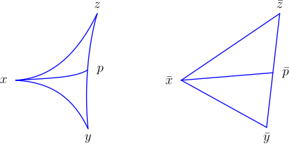
Curvature can be formulated in purely metric terms by comparing triangles with those in constant-curvature model spaces. For $\kappa \in \mathbb{R}$, let $\mathbb{M}_\kappa^2$ denote the complete simply connected two-dimensional space form of constant curvature $\kappa$: the Euclidean plane when $\kappa = 0$, the sphere of radius $1/\sqrt{\kappa}$ when $\kappa > 0$, and the hyperbolic plane when $\kappa < 0$.
Consider a geodesic triangle $\triangle(x, y, z)$ in $\mathcal{M}$. A **comparison triangle** in $\mathbb{M}_\kappa^2$ is a triangle $\overline{\triangle}(\bar{x}, \bar{y}, \bar{z})$ having the same side lengths,
$$
d(x, y) = d_\kappa(\bar{x}, \bar{y}), \quad d(y, z) = d_\kappa(\bar{y}, \bar{z}), \quad d(z, x) = d_\kappa(\bar{z}, \bar{x}),
$$
where $d_\kappa$ denotes the distance in $\mathbb{M}_\kappa^2$. When $\kappa > 0$, one restricts to sufficiently small triangles.
{width=80%}
::: {#def-cat-curvature .definition title="Global and local comparison curvature"}
Let
$$
D_\kappa = \begin{cases}
\pi / \sqrt{\kappa}, & \kappa > 0, \\
\infty, & \kappa \le 0.
\end{cases}
$$
A geodesic metric space $(\mathcal{M}, d)$ is called a **$\mathrm{CAT}(\kappa)$ space** if for every geodesic triangle $\triangle(x, y, z)$ with perimeter
$$
d(x, y) + d(y, z) + d(z, x) < 2D_\kappa,
$$
and for every comparison triangle $\overline{\triangle}(\bar{x}, \bar{y}, \bar{z})$ in $\mathbb{M}_\kappa^2$, the following holds: if $p$ lies on the side from $y$ to $z$ and $\bar{p}$ is its comparison point, then
$$
d(x, p) \le d_\kappa(\bar{x}, \bar{p}).
$$
:::
A metric space $\mathcal{M}$ is said to be a space with **curvature $\le \kappa$**, or **locally $\mathrm{CAT}(\kappa)$**, if every point of $\mathcal{M}$ has a geodesically convex $\mathrm{CAT}(\kappa)$ neighbourhood. A locally $\mathrm{CAT}(0)$ space may be said to have **non-positive curvature**; such spaces are also called **NPC spaces**.
If the inequality is reversed — $d(x, p) \ge d_\kappa(\bar{x}, \bar{p})$ — then we say $\mathcal{M}$ has curvature **bounded from below**, or curvature $\ge \kappa$.
::: {#def-hadamard-space .definition title="Hadamard space"}
A **Hadamard space** is a complete geodesic $\mathrm{CAT}(0)$ space.
:::
::: {.callout-note title="Exercise"}
Show that a Hadamard space is uniquely geodesic. (Hint: use the $\mathrm{CAT}(0)$ inequality.) <a href="javascript:void(0)" onclick="showSolution('l2-sol-4')" class="solution-link">📝 Show Solution</a>
:::
**Hadamard spaces behave in many respects like Hilbert spaces:** geodesics are unique, geodesically convex sets admit unique metric projections, and squared distance functions are convex along geodesics. These properties make statistical analysis on data from Hadamard spaces much more tractable.
### Examples of Curvature Behavior
| Space | Curvature | Notes |
|---|---|---|
| Sphere $\mathbb{S}^p$ | $\mathrm{CAT}(1)$ (positive) | Not Hadamard; antipodal points have many geodesics |
| SPD matrices (affine-invariant / log-Euclidean / log-Cholesky) | $\mathrm{CAT}(0)$ | Unbounded Hadamard space |
| BHV tree space | $\mathrm{CAT}(0)$ | Unbounded Hadamard space [@BilleraHolmesVogtmann2001] |
| $(\mathcal{P}_2(\mathbb{R}), W_2)$ | $\mathrm{CAT}(0)$ | Flat: isometric to convex subset of $L^2(0,1)$ [@PanaretosZemel2020; @Kloeckner2010] |
| $(\mathcal{P}_2(\mathbb{R}^p), W_2)$ for $p > 1$ | Curvature $\ge 0$ | Genuinely curved, nonnegative Alexandrov curvature [@Otto2001; @Lott2008] |
## Uniqueness in Hadamard Spaces
The Fréchet mean in Hadamard spaces, if it exists, is unique, due to Proposition 4.3 of @Sturm2003.
::: {#prp-sturm-uniqueness .proposition title="Uniqueness in Hadamard spaces (Sturm 2003, Proposition 4.3)"}
Let $(\mathcal{M}, d)$ be a Hadamard space and $X$ a random element on $\mathcal{M}$ such that $\mathbb{E}\,d(X, x) < \infty$ for some $x \in \mathcal{M}$. Fix $y \in \mathcal{M}$. Then there exists a unique point $\mu \in \mathcal{M}$ minimizing the uniformly convex continuous function
$$
G(z) = \mathbb{E}[d^2(X, z) - d^2(X, y)],
$$
and this minimizer is independent of $y$. If further $\mathbb{E}\,d^2(X, x) < \infty$ for some $x \in \mathcal{M}$, then
$$
\mu = \arg\min_{z \in \mathcal{M}} \mathbb{E}\,d^2(X, z),
$$
that is, $\mu$ is the **Fréchet mean** of $X$.
:::
::: {#cor-sample-frechet-hadamard .corollary}
The sample Fréchet mean exists and is unique in Hadamard spaces.
:::
To present the proof, we need notions of convexity on geodesic metric spaces.
::: {#def-convex-functions .definition title="Convex, strongly convex, and uniformly convex functions"}
Let $(\mathcal{M}, d)$ be a geodesic metric space and let $f : \mathcal{M} \to \mathbb{R}$.
- $f$ is **convex** if for every geodesic $\gamma : [0,1] \to \mathcal{M}$,
$$
f\bigl(\gamma(t)\bigr) \le (1-t)f\bigl(\gamma(0)\bigr) + t f\bigl(\gamma(1)\bigr), \qquad t \in [0,1].
$$
- Given $\lambda > 0$, $f$ is **$\lambda$-strongly convex** if for every geodesic $\gamma : [0,1] \to \mathcal{M}$,
$$
f\bigl(\gamma(t)\bigr) \le (1-t)f\bigl(\gamma(0)\bigr) + t f\bigl(\gamma(1)\bigr) - \frac{\lambda}{2}t(1-t)d^2\bigl(\gamma(0), \gamma(1)\bigr), \qquad t \in [0,1].
$$
- $f$ is **uniformly convex** if there exists a strictly increasing function $\eta : [0,\infty) \to [0,\infty)$ with $\eta(0) = 0$ such that for every geodesic $\gamma : [0,1] \to \mathcal{M}$,
$$
f\bigl(\gamma(1/2)\bigr) \le \frac{1}{2}f\bigl(\gamma(0)\bigr) + \frac{1}{2}f\bigl(\gamma(1)\bigr) - \eta\bigl(d(\gamma(0), \gamma(1))\bigr).
$$
:::
Clearly, a strongly convex function is also uniformly convex.
::: {#prp-sturm-minimizer .proposition title="Minimizer of a uniformly convex function (Sturm 2003, Proposition 1.7)"}
Let $(\mathcal{M}, d)$ be a complete geodesic space, and let $f : \mathcal{M} \to \mathbb{R}$ be uniformly convex and lower semicontinuous. Then there exists a unique point $\mu \in \mathcal{M}$ such that
$$
f(\mu) = \inf_{z \in \mathcal{M}} f(z).
$$
Equivalently, $\mu = \arg\min_{z \in \mathcal{M}} f(z)$.
:::
::: {.callout-note title="Lower Semicontinuity" collapse="true"}
A function $f : \mathcal{M} \to \mathbb{R}$ on a metric space $(\mathcal{M}, d)$ is **lower semicontinuous** (l.s.c.) at a point $x \in \mathcal{M}$ if
$$
f(x) \le \liminf_{n \to \infty} f(x_n)
$$
for every sequence $(x_n)$ converging to $x$. Equivalently, for every $\varepsilon > 0$ there exists $\delta > 0$ such that $f(y) > f(x) - \varepsilon$ whenever $d(x, y) < \delta$. The function $f$ is lower semicontinuous on $\mathcal{M}$ if it is l.s.c. at every point.
**Intuition.** While a continuous function cannot jump in either direction, a lower semicontinuous function may only jump **downwards**, never upwards. Equivalently, its sublevel sets $\{x : f(x) \le c\}$ are closed for every $c \in \mathbb{R}$.
**Why it matters here.** Lower semicontinuity is the minimal regularity condition needed for an optimization problem to attain its minimum on a compact set — a continuous function is automatically l.s.c., but l.s.c. is enough.
:::
::: {#prp-sturm-convexity .proposition title="Geodesics and convexity of squared distance in Hadamard spaces (Sturm 2003, Proposition 2.3)"}
If $(\mathcal{M}, d)$ is a Hadamard space, then for each pair of points $x_0, x_1 \in \mathcal{M}$ there exists a unique geodesic $t \mapsto x_t$ on $[0,1]$ joining them. For each fixed $t \in [0,1]$, the point $x_t$ depends continuously on the endpoints $x_0, x_1$. Moreover, for every $z \in \mathcal{M}$ and every $t \in [0,1]$,
$$
d^2(z, x_t) \le (1-t)d^2(z, x_0) + t d^2(z, x_1) - t(1-t)d^2(x_0, x_1).
$$
:::
Therefore, for any fixed $z$, the squared distance function $f(x) = d^2(z, x)$ is **strongly convex** in a Hadamard space.
**Proof of [Proposition 2.1](#prp-sturm-uniqueness).** Let $q$ denote the law of $X$, and for fixed $y \in \mathcal{M}$ define
$$
F_y(z) = \int_{\mathcal{M}} \bigl[d^2(z, u) - d^2(y, u)\bigr]\,q(du) = \mathbb{E}\bigl[d^2(X, z) - d^2(X, y)\bigr].
$$
Then $F_y = G$. If $y_0 \in \mathcal{M}$ is another base point, then
$$
F_y(z) - F_{y_0}(z) = \int_{\mathcal{M}} \bigl[d^2(y_0, u) - d^2(y, u)\bigr]\,q(du),
$$
which is independent of $z$. Hence any minimizer is independent of the choice of $y$.
Now let $z_0, z_1 \in \mathcal{M}$ and let $z_t$ be the geodesic joining them. By the squared-distance convexity proposition, for every $u \in \mathcal{M}$,
$$
d^2(z_t, u) \le (1-t)d^2(z_0, u) + t d^2(z_1, u) - t(1-t)d^2(z_0, z_1),
$$
or equivalently,
$$
d^2(z_t, u) - d^2(y, u) \le (1-t)[d^2(z_0, u) - d^2(y, u)] + t[d^2(z_1, u) - d^2(y, u)] - t(1-t)d^2(z_0, z_1).
$$
Integrating with respect to $q$ yields
$$
F_y(z_t) \le (1-t)F_y(z_0) + t F_y(z_1) - t(1-t)d^2(z_0, z_1),
$$
so $F_y$ is strongly convex and thus uniformly convex. Moreover,
$$
|F_y(z) - F_y(z_0)| \le d(z, z_0)\int_{\mathcal{M}} \bigl(d(z, u) + d(z_0, u)\bigr)\,q(du),
$$
so $F_y$ is continuous. Therefore $F_y$ has a unique minimizer on the Hadamard space $\mathcal{M}$.
If in addition $\mathbb{E}\,d^2(X, x) < \infty$, then
$$
F_y(z) = \mathbb{E}\,d^2(X, z) - \mathbb{E}\,d^2(X, y)
$$
differs from $z \mapsto \mathbb{E}\,d^2(X, z)$ only by an additive constant. Thus they have the same unique minimizer — the Fréchet mean of $X$. □
## Application: Fréchet Mean of Covariance Matrices for Portfolio Risk
Covariance matrices are central to portfolio theory and risk management. The variance of a portfolio with weight vector $w \in \mathbb{R}^p$ is
$$
\operatorname{Var}(w^\top R) = w^\top \Sigma w,
$$
where $\Sigma \in \mathcal{S}_{++}^{p}$ is the covariance matrix of asset returns. Covariance matrices live not in $\mathbb{R}^{p \times p}$ but in the **cone of symmetric positive definite (SPD) matrices** — a non-Euclidean space with its own curved geometry [@BhattacharyaPatrangenaru2003; @PennecFillardAyache2006].
**A natural question arises:** if we observe covariance matrices $\Sigma_1, \Sigma_2, \ldots, \Sigma_n$ estimated from rolling time windows, what is the "average market risk structure"? The ordinary Euclidean average
$$
\bar{\Sigma}_{\text{Euclid}} = \frac{1}{n}\sum_{i=1}^n \Sigma_i
$$
is a valid SPD matrix (the SPD cone is convex in the Euclidean sense), but it ignores the intrinsic geometry of $\mathcal{S}_{++}^{p}$. Two geometrically motivated alternatives are:
1. **Log-Euclidean Fréchet mean** [@ArsignyEtAl2006]: map each $\Sigma_i$ to the tangent space at the identity via the matrix logarithm, average in that flat space, and map back:
$$
\hat{\Sigma}_{\mathrm{LE}} = \exp\!\left(\frac{1}{n}\sum_{i=1}^n \log(\Sigma_i)\right).
$$
This is the unique Fréchet mean under the log-Euclidean metric $d_{\mathrm{LE}}(\Sigma_1, \Sigma_2) = \|\log(\Sigma_1) - \log(\Sigma_2)\|_F$.
2. **Affine-invariant Riemannian Fréchet mean** [@PennecFillardAyache2006; @Moakher2005GeometricMean]: the intrinsic mean under the affine-invariant metric $d_{\mathrm{AI}}(\Sigma_1, \Sigma_2) = \|\log(\Sigma_1^{-1/2}\Sigma_2\Sigma_1^{-1/2})\|_F$. This metric is invariant under congruence transformations $\Sigma \mapsto A\Sigma A^\top$, making it particularly natural for covariance matrices. Its Fréchet mean has no closed form and requires iterative computation.
The log-Euclidean and affine-invariant means both respect the SPD cone geometry, unlike the Euclidean mean which can produce "swelling" artifacts (inflated determinants) and does not preserve the natural Riemannian structure.
The demo below generates synthetic monthly covariance matrices for three assets (modeled on AAPL, MSFT, and JPM). Each matrix corresponds to a different market regime (turbulent, calm, tech-rally, etc.). Adjust the seed to explore different realizations, then compare the Euclidean and log-Euclidean Fréchet means.
<script src="https://cdn.jsdelivr.net/npm/[email protected]/lib/browser/math.js"></script>
<div id="portfolio-risk-demo" style="border:1px solid #ddd; border-radius:8px; padding:1rem; background:#fcfcfc; margin:1rem 0;">
<div style="display:flex; gap:1rem; align-items:center; flex-wrap:wrap; margin-bottom:1rem;">
<label style="font-weight:600;">
Seed:
<input id="pr-seed" type="number" value="42" min="1" max="9999" style="width:5rem; margin-left:0.3rem;">
</label>
<button id="pr-generate" style="padding:0.3rem 0.8rem; cursor:pointer; font-weight:600; background:#5b9bd5; color:white; border:none; border-radius:4px;">Regenerate</button>
<span style="color:#888; font-size:0.85rem;" id="pr-meta"></span>
</div>
<div id="pr-matrices-grid" style="display:flex; flex-wrap:wrap; gap:0.5rem; margin-bottom:1rem;"></div>
<div id="pr-means-panel" style="display:flex; gap:1.5rem; flex-wrap:wrap;"></div>
<div id="pr-interpretation" style="margin-top:0.75rem; padding:0.5rem 0.75rem; background:#f0f4f8; border-radius:6px; font-size:0.9rem;"></div>
</div>
<script>
(function() {
// --- Seeded PRNG (mulberry32) ---
function mulberry32(a) {
return function() {
a |= 0; a = a + 0x6D2B79F5 | 0;
var t = Math.imul(a ^ a >>> 15, 1 | a);
t = t + Math.imul(t ^ t >>> 7, 61 | t) ^ t;
return ((t ^ t >>> 14) >>> 0) / 4294967296;
};
}
function eigScalar(x) {
if (typeof x === 'number') return x;
if (x && typeof x.re === 'number') return x.re;
return Number(x);
}
function eigVectorArray(v) {
var arr = v && v.toArray ? v.toArray() : v;
return arr.map(eigScalar);
}
function symmetricEigensystem(M) {
var eig = math.eigs(M);
if (eig.eigenvectors && eig.eigenvectors[0] && eig.eigenvectors[0].vector) {
var columns = eig.eigenvectors.map(function(e) { return eigVectorArray(e.vector); });
return {
values: eig.eigenvectors.map(function(e) { return eigScalar(e.value); }),
vectors: math.transpose(math.matrix(columns))
};
}
return {
values: eig.values.map(eigScalar),
vectors: math.matrix(eig.eigenvectors || eig.vectors)
};
}
// --- Matrix logarithm via eigendecomposition ---
function matLog(M) {
var eig = symmetricEigensystem(M);
var vals = eig.values;
var vecs = eig.vectors;
var logVals = math.diag(vals.map(function(v) { return Math.log(Math.max(v, 1e-12)); }));
return math.multiply(vecs, math.multiply(logVals, math.transpose(vecs)));
}
// --- Matrix exponential via eigendecomposition ---
function matExp(M) {
var eig = symmetricEigensystem(M);
var vals = eig.values;
var vecs = eig.vectors;
var expVals = math.diag(vals.map(function(v) { return Math.exp(v); }));
return math.multiply(vecs, math.multiply(expVals, math.transpose(vecs)));
}
// --- Frobenius norm ---
function frobNorm(M) {
var a = (M.toArray ? M.toArray() : M);
var s = 0;
for (var i = 0; i < a.length; i++)
for (var j = 0; j < a[i].length; j++)
s += a[i][j] * a[i][j];
return Math.sqrt(s);
}
// --- Labels ---
var labels = ['AAPL', 'MSFT', 'JPM'];
// --- Random orthogonal matrix (via QR decomposition) ---
function randomOrthogonal(rng) {
var a = [[], [], []];
for (var i = 0; i < 3; i++)
for (var j = 0; j < 3; j++)
a[i][j] = (rng() - 0.5) * 2; // fill [-1, 1]
var qr = math.qr(math.matrix(a));
return qr.Q;
}
// --- Generate random SPD with skewed eigenvalues ---
// Each Σ = R Λ Rᵀ where R is a random orthogonal matrix (so the dominant
// eigenvector can point in any direction) and Λ = diag(λ₁, λ₂, λ₃) has
// skewed entries: λ₁ ≫ λ₂ ≫ λ₃ in many draws (condition numbers up to ~30).
// The eigenvalues are scaled so det(Σ) ≈ 0.01.
function randomSPD(rng) {
// Raw skewed eigenvalues — large, medium, small
var raw1 = 0.40 + rng() * 0.35; // largest: 0.40 – 0.75
var raw2 = 0.08 + rng() * 0.20; // medium: 0.08 – 0.28
var raw3 = 0.02 + rng() * 0.10; // smallest: 0.02 – 0.12
// Scale to keep determinant in the neighbourhood of 0.01
var rawDet = raw1 * raw2 * raw3;
var targetDet = 0.006 + rng() * 0.020; // 0.006 – 0.026
var scale = Math.cbrt(targetDet / rawDet);
var eigs = [raw1 * scale, raw2 * scale, raw3 * scale];
// Random eigenvectors (the dominant direction is uniformly distributed)
var R = randomOrthogonal(rng);
var D = math.diag(eigs);
return math.multiply(R, math.multiply(D, math.transpose(R)));
}
// --- Render matrix as colored table ---
function matrixTable(M, hl) {
var arr = M.toArray();
var maxAbs = 0;
for (var i = 0; i < 3; i++)
for (var j = 0; j < 3; j++)
maxAbs = Math.max(maxAbs, Math.abs(arr[i][j]));
if (maxAbs === 0) maxAbs = 1;
var h = '<table style="font-size:0.78rem; border-collapse:collapse;">';
h += '<tr><td></td>' + labels.map(function(l) { return '<td style="padding:1px 5px;font-weight:600;font-size:0.7rem;color:#555;">'+l+'</td>'; }).join('') + '</tr>';
for (var i = 0; i < 3; i++) {
h += '<tr><td style="padding:1px 5px;font-weight:600;font-size:0.7rem;color:#555;">' + labels[i] + '</td>';
for (var j = 0; j < 3; j++) {
var v = arr[i][j];
var intensity = Math.round(255 * (1 - Math.abs(v) / (maxAbs * 1.05)));
var bg;
if (v >= 0) bg = 'rgb(255,' + intensity + ',' + intensity + ')';
else bg = 'rgb(' + intensity + ',' + intensity + ',255)';
var fw = hl && hl[0] === i && hl[1] === j ? 'font-weight:900;' : '';
h += '<td style="padding:2px 6px;text-align:right;background:' + bg + ';' + fw + '">' + v.toFixed(4) + '</td>';
}
h += '</tr>';
}
h += '</table>';
return h;
}
// --- Main render ---
function render() {
if (!window.math) {
document.getElementById('pr-meta').textContent = 'Loading matrix library...';
return;
}
var seed = parseInt(document.getElementById('pr-seed').value) || 42;
var rng = mulberry32(seed);
var nMat = 8;
var nAssets = 3;
// Generate matrices
var matrices = [];
for (var k = 0; k < nMat; k++) {
matrices.push(randomSPD(rng));
}
// --- Euclidean mean ---
var sumE = math.zeros(3, 3);
for (var k = 0; k < nMat; k++) sumE = math.add(sumE, matrices[k]);
var euclidMean = math.multiply(sumE, 1 / nMat);
// --- Log-Euclidean Fréchet mean ---
var sumLog = math.zeros(3, 3);
var logs = [];
for (var k = 0; k < nMat; k++) {
var L = matLog(matrices[k]);
logs.push(L);
sumLog = math.add(sumLog, L);
}
var meanLog = math.multiply(sumLog, 1 / nMat);
var leMean = matExp(meanLog);
var dEuclid = math.det(euclidMean);
var dLE = math.det(leMean);
var frobDist = frobNorm(math.subtract(euclidMean, leMean));
// --- Render matrices grid ---
var regimeNames = ['Calm', 'Turbulent', 'Tech rally', 'Risk-off', 'Recovery', 'High vol', 'Low vol', 'Stressed'];
var gridHtml = '';
for (var k = 0; k < nMat; k++) {
gridHtml += '<div style="border:1px solid #e0e0e0;border-radius:6px;padding:0.4rem 0.55rem;background:#fff;">' +
'<div style="font-weight:700;font-size:0.8rem;margin-bottom:0.25rem;">Σ<sub>' + (k+1) + '</sub> <span style="font-weight:400;color:#999;">' + regimeNames[k] + '</span></div>' +
matrixTable(matrices[k]) +
'<div style="font-size:0.7rem;color:#999;margin-top:0.2rem;">det: ' + math.det(matrices[k]).toFixed(4) + '</div>' +
'</div>';
}
document.getElementById('pr-matrices-grid').innerHTML = gridHtml;
// --- Render means ---
var meansHtml = '' +
'<div style="border:2px solid #3498db;border-radius:8px;padding:0.75rem;background:#fff;flex:1;min-width:220px;">' +
'<div style="font-weight:700;color:#3498db;margin-bottom:0.4rem;">Euclidean Mean</div>' +
matrixTable(euclidMean) +
'<div style="font-size:0.8rem;margin-top:0.3rem;">det = <strong>' + dEuclid.toFixed(4) + '</strong></div>' +
'<div style="font-size:0.75rem;color:#888;">arithmetic average of Σ<sub>i</sub></div>' +
'</div>' +
'<div style="border:2px solid #27ae60;border-radius:8px;padding:0.75rem;background:#fff;flex:1;min-width:220px;">' +
'<div style="font-weight:700;color:#27ae60;margin-bottom:0.4rem;">Log-Euclidean Fréchet Mean</div>' +
matrixTable(leMean) +
'<div style="font-size:0.8rem;margin-top:0.3rem;">det = <strong>' + dLE.toFixed(4) + '</strong></div>' +
'<div style="font-size:0.75rem;color:#888;">exp(mean(log Σ<sub>i</sub>))</div>' +
'</div>';
document.getElementById('pr-means-panel').innerHTML = meansHtml;
// --- Interpretation ---
var detRatio = dEuclid / dLE;
// Find the maximum determinant among individual matrices
var maxIndivDet = 0;
for (var k = 0; k < nMat; k++) {
var dk = math.det(matrices[k]);
if (dk > maxIndivDet) maxIndivDet = dk;
}
var swellRatio = dEuclid / maxIndivDet;
var interpHtml = '<strong>🔍 Observation:</strong> ';
if (detRatio > 1.05) {
interpHtml += 'The Euclidean mean has a <strong>' + detRatio.toFixed(1) + '× larger determinant</strong> than the log-Euclidean Fréchet mean — this is the "swelling" effect. ';
} else if (detRatio < 0.95) {
interpHtml += 'The Euclidean mean has a <strong>smaller determinant</strong> than the log-Euclidean mean in this realization. ';
} else {
interpHtml += 'Both means have similar determinants in this realization. ';
}
interpHtml += 'The Frobenius distance between the two means is <strong>' + frobDist.toFixed(4) + '</strong>. ';
if (swellRatio > 1.01) {
interpHtml += 'Notably, det(Euclidean mean) = <strong>' + dEuclid.toFixed(4) + '</strong> exceeds <em>every</em> individual det (max = ' + maxIndivDet.toFixed(4) + '), a ' + swellRatio.toFixed(1) + '× inflation — the arithmetic average spuriously amplifies the overall market risk. ';
} else if (swellRatio < 0.99) {
interpHtml += 'In this draw the Euclidean mean happens to have a smaller determinant than the largest individual matrix (det = ' + maxIndivDet.toFixed(4) + '); re-running with a different seed usually restores the swelling pattern. ';
} else {
interpHtml += 'The Euclidean and the largest individual determinants are nearly equal in this realization. ';
}
interpHtml += 'The log-Euclidean mean averages in the log-domain (where matrices form a vector space), respecting the multiplicative structure of the SPD cone. ';
interpHtml += 'This can have material implications for portfolio optimization: the log-Euclidean mean typically yields <strong>more conservative risk estimates</strong>, avoiding the variance-inflation bias of the arithmetic average.';
document.getElementById('pr-interpretation').innerHTML = interpHtml;
document.getElementById('pr-meta').textContent = nMat + ' covariance matrices, ' + nAssets + ' assets';
}
// --- Boot ---
function nextSeed() {
var seedInput = document.getElementById('pr-seed');
var current = parseInt(seedInput.value) || 42;
var next = (current % 9999) + 1;
seedInput.value = next;
render();
}
function boot() {
if (!window.math) {
document.getElementById('pr-meta').textContent = 'Loading matrix library...';
setTimeout(boot, 100);
return;
}
render();
document.getElementById('pr-generate').addEventListener('click', nextSeed);
document.getElementById('pr-seed').addEventListener('change', render);
}
if (document.readyState === 'loading') {
document.addEventListener('DOMContentLoaded', boot);
} else {
boot();
}
})();
</script>
**Observations**
- The **Euclidean mean** of SPD matrices can inflate variances and correlations — the SPD cone geometry is not flat.
- The **log-Euclidean Fréchet mean** respects the multiplicative structure: variances and covariances are averaged geometrically via the matrix logarithm.
- In practice, the choice of metric for averaging covariance matrices affects **portfolio risk estimates**, **diversification measures**, and **regulatory capital calculations**.
- The **affine-invariant Fréchet mean** goes further by ensuring invariance under changes of basis (e.g., currency conversions or factor rotations), but at the cost of requiring iterative computation [@PennecFillardAyache2006].
## Key Takeaways
- The **Fréchet mean** generalizes the Euclidean mean by minimizing expected squared distance.
- In arbitrary metric spaces, Fréchet means may **fail to exist** or may not be **unique**.
- The **Heine–Borel property** (closed bounded sets are compact) guarantees existence.
- **Hadamard spaces** — complete geodesic $\mathrm{CAT}(0)$ spaces — guarantee **uniqueness**.
- The squared distance function in a Hadamard space is **strongly convex** along geodesics, which is the key geometric fact behind uniqueness.
- Key examples of Hadamard spaces: SPD matrices (under intrinsic metrics), BHV tree space, and the 1D Wasserstein space.
## Exercises
1. **Finiteness of the Fréchet function**: Prove that if $\mathbb{E}\{d^2(X, x_0)\} < \infty$ for some $x_0 \in \mathcal{M}$, then $\mathbb{E}\{d^2(X, x)\} < \infty$ for all $x \in \mathcal{M}$. <a href="javascript:void(0)" onclick="showSolution('l2-sol-1')" class="solution-link">📝 Show Solution</a>
2. **Non-uniqueness on the sphere**: Let $X$ be uniformly distributed on $\mathbb{S}^p$. Show that $F(x)$ is constant on $\mathbb{S}^p$, so every point is a Fréchet mean. (Hint: use rotational symmetry.) <a href="javascript:void(0)" onclick="showSolution('l2-sol-2')" class="solution-link">📝 Show Solution</a>
3. **Boundedness of $S_c$**: In the proof of [Theorem 2.1](#thm-heine-borel), show that the set $S_c = \{x \in \mathcal{M} : F(x) \le c\}$ is bounded. <a href="javascript:void(0)" onclick="showSolution('l2-sol-3')" class="solution-link">📝 Show Solution</a>
4. **Hadamard spaces are uniquely geodesic**: Prove that a Hadamard space is uniquely geodesic. (Hint: use the $\mathrm{CAT}(0)$ inequality.) <a href="javascript:void(0)" onclick="showSolution('l2-sol-4')" class="solution-link">📝 Show Solution</a>
5. **Strong convexity of squared distance**: Verify that in $\mathbb{R}^p$ with the Euclidean metric, the squared-distance convexity inequality holds with equality (in fact, it's the parallelogram law in disguise). <a href="javascript:void(0)" onclick="showSolution('l2-sol-5')" class="solution-link">📝 Show Solution</a>
6. **Comparison triangle construction**: For three points in $\mathbb{R}^2$ with the Euclidean metric, construct their comparison triangle. Show that $d(x, p) = d_0(\bar{x}, \bar{p})$ — there is no distortion. <a href="javascript:void(0)" onclick="showSolution('l2-sol-6')" class="solution-link">📝 Show Solution</a>
<style>
.solution-link {
font-size: 0.9em;
text-decoration: none;
white-space: nowrap;
margin-left: 0.3em;
}
.solution-link:hover {
text-decoration: underline;
}
.solution-dialog {
padding: 0;
max-width: 720px;
}
.solution-dialog-header {
display: flex;
justify-content: space-between;
align-items: flex-start;
border-bottom: 1px solid #dee2e6;
padding: 1.25rem 1.5rem 1rem;
background: #f8f9fa;
border-radius: 8px 8px 0 0;
}
.solution-dialog-header h4 {
margin: 0;
font-size: 1.15rem;
}
.solution-dialog-close {
background: none;
border: 1px solid #adb5bd;
border-radius: 4px;
padding: 0.2rem 0.75rem;
cursor: pointer;
font-size: 0.9rem;
color: #495057;
white-space: nowrap;
flex-shrink: 0;
}
.solution-dialog-close:hover {
background: #e9ecef;
}
.solution-original {
padding: 1rem 1.5rem;
background: #f1f3f5;
border-left: 4px solid #868e96;
margin: 1rem 1.5rem;
border-radius: 4px;
font-size: 0.95rem;
}
.solution-original strong {
color: #495057;
}
.solution-answer {
padding: 0.5rem 1.5rem 1.5rem;
}
.solution-answer strong {
color: #2b8a3e;
}
dialog {
border: none;
border-radius: 8px;
box-shadow: 0 8px 32px rgba(0,0,0,0.22);
padding: 0;
max-width: 750px;
width: 90vw;
}
dialog::backdrop {
background: rgba(0,0,0,0.45);
}
</style>
<dialog id="l2-sol-1">
<div class="solution-dialog">
<div class="solution-dialog-header">
<h4>Exercise 1: Finiteness of the Fréchet Function</h4>
<button onclick="closeSolution('l2-sol-1')" class="solution-dialog-close">✕ Close</button>
</div>
<div class="solution-original">
<strong>Exercise:</strong> Prove that if $\mathbb{E}\{d^2(X, x_0)\} < \infty$ for some $x_0 \in \mathcal{M}$, then $\mathbb{E}\{d^2(X, x)\} < \infty$ for all $x \in \mathcal{M}$.
</div>
<div class="solution-answer">
<strong>Solution:</strong>
By the triangle inequality, for any $x, x_0 \in \mathcal{M}$,
$$d(X, x) \le d(X, x_0) + d(x_0, x).$$
Squaring both sides and using the inequality $(a+b)^2 \le 2a^2 + 2b^2$ (which follows from $(a-b)^2 \ge 0$),
$$d^2(X, x) \le \bigl(d(X, x_0) + d(x_0, x)\bigr)^2 \le 2\,d^2(X, x_0) + 2\,d^2(x_0, x).$$
Taking expectations,
$$\mathbb{E}\,d^2(X, x) \le 2\,\mathbb{E}\,d^2(X, x_0) + 2\,d^2(x_0, x).$$
Since $\mathbb{E}\,d^2(X, x_0) < \infty$ by assumption and $d(x_0, x)$ is a finite constant (not random), the right-hand side is finite. Therefore $\mathbb{E}\,d^2(X, x) < \infty$ for all $x \in \mathcal{M}$.
This simple observation ensures that the Fréchet function $F(x) = \mathbb{E}\,d^2(X, x)$ is well-defined on the whole space whenever it is finite at a single point.
</div>
</div>
</dialog>
<dialog id="l2-sol-2">
<div class="solution-dialog">
<div class="solution-dialog-header">
<h4>Exercise 2: Non-Uniqueness on the Sphere</h4>
<button onclick="closeSolution('l2-sol-2')" class="solution-dialog-close">✕ Close</button>
</div>
<div class="solution-original">
<strong>Exercise:</strong> Let $X$ be uniformly distributed on $\mathbb{S}^p$. Show that $F(x)$ is constant on $\mathbb{S}^p$, so every point is a Fréchet mean.
</div>
<div class="solution-answer">
<strong>Solution:</strong>
Let $X \sim \operatorname{Uniform}(\mathbb{S}^p)$. The distribution of $X$ is invariant under the action of the orthogonal group $O(p+1)$: for any $R \in O(p+1)$, the random variable $R X$ has the same distribution as $X$, because the uniform measure on the sphere is the unique rotationally-invariant probability measure.
Now fix any two points $x, y \in \mathbb{S}^p$. Since $O(p+1)$ acts transitively on the sphere, there exists a rotation $R \in O(p+1)$ such that $y = R x$. Then
\begin{align*}
F(y) = F(R x) &= \mathbb{E}\bigl[d^2(X, R x)\bigr] \\
&= \mathbb{E}\bigl[d^2(R^{-1} X, x)\bigr] \quad \text{(since } R \text{ is an isometry)} \\
&= \mathbb{E}\bigl[d^2(X, x)\bigr] \quad \text{(since } R^{-1}X \stackrel{d}{=} X \text{ by rotational invariance)} \\
&= F(x).
\end{align*}
Thus $F(x) = F(y)$ for all $x, y \in \mathbb{S}^p$ — the Fréchet function is constant. Since every point attains the same value, every point is a minimizer, and hence every point on the sphere is a Fréchet mean.
</div>
</div>
</dialog>
<dialog id="l2-sol-3">
<div class="solution-dialog">
<div class="solution-dialog-header">
<h4>Exercise 3: Boundedness of $S_c$</h4>
<button onclick="closeSolution('l2-sol-3')" class="solution-dialog-close">✕ Close</button>
</div>
<div class="solution-original">
<strong>Exercise:</strong> In the proof of [Theorem 2.1](#thm-heine-borel), show that the set $S_c = \{x \in \mathcal{M} : F(x) \le c\}$ is bounded.
</div>
<div class="solution-answer">
<strong>Solution:</strong>
Let $x_0 \in \mathcal{M}$ be any fixed point. For any $x \in S_c$, we bound $d(x_0, x)$ as follows.
First, by the triangle inequality, $d(x_0, x) \le d(x_0, X) + d(X, x)$. Squaring and using $(a+b)^2 \le 2a^2 + 2b^2$:
$$d^2(x_0, x) \le 2\,d^2(X, x_0) + 2\,d^2(X, x).$$
Now take expectations:
\begin{align*}
d^2(x_0, x) &= \mathbb{E}\,d^2(x_0, x) \quad \text{(left side is deterministic)} \\
&\le 2\,\mathbb{E}\,d^2(X, x_0) + 2\,\mathbb{E}\,d^2(X, x) \\
&= 2F(x_0) + 2F(x).
\end{align*}
Since $x \in S_c$, we have $F(x) \le c$. Therefore
$$d^2(x_0, x) \le 2F(x_0) + 2c.$$
Taking square roots,
$$d(x_0, x) \le \sqrt{2F(x_0) + 2c}.$$
This uniform bound holds for every $x \in S_c$. Hence $S_c$ is contained in the closed ball of radius $R = \sqrt{2F(x_0) + 2c}$ centered at $x_0$, and is therefore bounded.
</div>
</div>
</dialog>
<dialog id="l2-sol-4">
<div class="solution-dialog">
<div class="solution-dialog-header">
<h4>Exercise 4: Hadamard Spaces Are Uniquely Geodesic</h4>
<button onclick="closeSolution('l2-sol-4')" class="solution-dialog-close">✕ Close</button>
</div>
<div class="solution-original">
<strong>Exercise:</strong> Prove that a Hadamard space is uniquely geodesic. (Hint: use the $\mathrm{CAT}(0)$ inequality.)
</div>
<div class="solution-answer">
<strong>Solution:</strong>
Let $(\mathcal{M}, d)$ be a Hadamard space (a complete geodesic $\mathrm{CAT}(0)$ space). Because it is geodesic, at least one geodesic joins every pair of points. It remains to prove uniqueness.
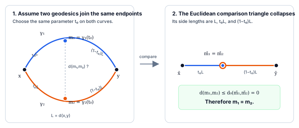
Suppose that two geodesics $\gamma_1, \gamma_2 : [0,1] \to \mathcal{M}$ have the same endpoints:
$$\gamma_1(0) = \gamma_2(0) = x, \qquad \gamma_1(1) = \gamma_2(1) = y.$$
Fix any $t_0 \in (0,1)$ and set
$$m_1 = \gamma_1(t_0), \qquad m_2 = \gamma_2(t_0), \qquad L=d(x,y).$$
The picture shows the only apparent way the two geodesics could differ, and why the $\mathrm{CAT}(0)$ comparison rules it out.
{width=100%}
Now consider the geodesic triangle $\triangle(x, y, m_2)$ whose side from $x$ to $y$ is $\gamma_1$, while its other two sides are the corresponding subsegments of $\gamma_2$. Construct its comparison triangle $\overline{\triangle}(\bar{x}, \bar{y}, \bar{m}_2)$ in the Euclidean plane $\mathbb{R}^2$ (the model space $\mathbb{M}_0^2$). The comparison triangle has side lengths:
$$d_0(\bar{x}, \bar{y}) = L, \quad d_0(\bar{x}, \bar{m}_2) = t_0L, \quad d_0(\bar{m}_2, \bar{y}) = (1-t_0)L.$$
These lengths add with equality: $t_0L+(1-t_0)L=L$. Consequently the comparison triangle is degenerate, with $\bar{m}_2$ at parameter $t_0$ on the segment from $\bar{x}$ to $\bar{y}$.
The point $m_1$ lies at the same parameter $t_0$ on the other side from $x$ to $y$. Its comparison point $\bar{m}_1$ therefore also lies at parameter $t_0$ on $\bar{x}\bar{y}$. Hence $\bar{m}_1=\bar{m}_2$.
By the $\mathrm{CAT}(0)$ inequality applied to the triangle $\triangle(x, y, m_2)$ with the point $m_1$ on the side $xy$,
$$d(m_2,m_1)\le d_0(\bar{m}_2,\bar{m}_1)=0.$$
Thus $\gamma_1(t_0)=\gamma_2(t_0)$. Since $t_0$ was arbitrary (and the endpoints already agree), $\gamma_1(t)=\gamma_2(t)$ for every $t\in[0,1]$.
Thus geodesics in a Hadamard space are unique.
</div>
</div>
</dialog>
<dialog id="l2-sol-5">
<div class="solution-dialog">
<div class="solution-dialog-header">
<h4>Exercise 5: Strong Convexity of Squared Distance in $\mathbb{R}^p$</h4>
<button onclick="closeSolution('l2-sol-5')" class="solution-dialog-close">✕ Close</button>
</div>
<div class="solution-original">
<strong>Exercise:</strong> Verify that in $\mathbb{R}^p$ with the Euclidean metric, the squared-distance convexity inequality holds with equality (in fact, it's the parallelogram law in disguise).
</div>
<div class="solution-answer">
<strong>Solution:</strong>
In $\mathbb{R}^p$, the geodesic from $x_0$ to $x_1$ is $\gamma(t) = x_t = (1-t)x_0 + t x_1$. For any $z \in \mathbb{R}^p$, we compute:
\begin{align*}
d^2(z, x_t) &= \|z - x_t\|^2 = \|z - (1-t)x_0 - t x_1\|^2 \\
&= \|(1-t)(z - x_0) + t(z - x_1)\|^2 \\
&= (1-t)^2\|z - x_0\|^2 + t^2\|z - x_1\|^2 + 2t(1-t)\langle z - x_0, z - x_1 \rangle.
\end{align*}
On the other hand,
\begin{align*}
&(1-t)d^2(z, x_0) + t d^2(z, x_1) - t(1-t)d^2(x_0, x_1) \\
&= (1-t)\|z-x_0\|^2 + t\|z-x_1\|^2 - t(1-t)\|x_0 - x_1\|^2.
\end{align*}
The difference is:
\begin{align*}
&\bigl[(1-t) - (1-t)^2\bigr]\|z-x_0\|^2 + \bigl[t - t^2\bigr]\|z-x_1\|^2 \\
&\qquad - 2t(1-t)\langle z-x_0, z-x_1 \rangle - t(1-t)\|x_0-x_1\|^2 \\
&= t(1-t)\Bigl[\|z-x_0\|^2 + \|z-x_1\|^2 - 2\langle z-x_0, z-x_1 \rangle - \|x_0-x_1\|^2\Bigr].
\end{align*}
Now observe:
\begin{align*}
\|z-x_0\|^2 + \|z-x_1\|^2 - 2\langle z-x_0, z-x_1 \rangle
&= \|(z-x_0) - (z-x_1)\|^2 \\
&= \|x_1 - x_0\|^2 = \|x_0 - x_1\|^2.
\end{align*}
Therefore the difference is $t(1-t)[\|x_0-x_1\|^2 - \|x_0-x_1\|^2] = 0$, and we have:
$$d^2(z, x_t) = (1-t)d^2(z, x_0) + t d^2(z, x_1) - t(1-t)d^2(x_0, x_1).$$
The convexity inequality holds with **equality** in Euclidean space. This is indeed a disguised form of the parallelogram law: the "gap" $t(1-t)d^2(x_0, x_1)$ exactly accounts for the curvature of the squared-distance function along the geodesic. In positively curved spaces, the gap is smaller; in negatively curved (Hadamard) spaces, the gap is larger, which is what drives the strong convexity used in the uniqueness proof.
</div>
</div>
</dialog>
<dialog id="l2-sol-6">
<div class="solution-dialog">
<div class="solution-dialog-header">
<h4>Exercise 6: Comparison Triangle in Euclidean Space</h4>
<button onclick="closeSolution('l2-sol-6')" class="solution-dialog-close">✕ Close</button>
</div>
<div class="solution-original">
<strong>Exercise:</strong> For three points in $\mathbb{R}^2$ with the Euclidean metric, construct their comparison triangle. Show that $d(x, p) = d_0(\bar{x}, \bar{p})$ — there is no distortion.
</div>
<div class="solution-answer">
<strong>Solution:</strong>
Let $x, y, z \in \mathbb{R}^2$ be three points forming a geodesic triangle $\triangle(x, y, z)$. The comparison triangle $\overline{\triangle}(\bar{x}, \bar{y}, \bar{z})$ in the model space $\mathbb{M}_0^2 = \mathbb{R}^2$ is any triangle with the same side lengths:
$$d(\bar{x}, \bar{y}) = d(x, y), \quad d(\bar{y}, \bar{z}) = d(y, z), \quad d(\bar{z}, \bar{x}) = d(z, x).$$
Since both the original triangle and the comparison triangle lie in $\mathbb{R}^2$ and have identical side lengths, they are **congruent** — there exists a rigid motion (translation + rotation + possibly reflection) mapping one to the other. Without loss of generality, we may take $\bar{x} = x$, $\bar{y} = y$, $\bar{z} = z$.
Now let $p$ be a point on the geodesic from $y$ to $z$, say $p = (1-s)y + s z$ for some $s \in [0,1]$. Its comparison point $\bar{p}$ on the side $\bar{y}\bar{z}$ is $\bar{p} = (1-s)\bar{y} + s\bar{z} = (1-s)y + s z = p$.
Therefore $d(x, p) = \|\bar{x} - \bar{p}\| = d_0(\bar{x}, \bar{p})$, and the $\mathrm{CAT}(0)$ inequality
$$d(x, p) \le d_0(\bar{x}, \bar{p})$$
holds with **equality**. There is no distortion because Euclidean space is itself the model space for $\kappa = 0$.
This is the defining property of $\mathrm{CAT}(0)$ spaces: triangles are "at least as thin" as their Euclidean comparison triangles. Euclidean space itself saturates this bound exactly, while negatively curved spaces have strictly thinner triangles ($d(x, p) < d_0(\bar{x}, \bar{p})$), and positively curved spaces violate the inequality.
</div>
</div>
</dialog>
<dialog id="l2-sol-frechet-equals-mean">
<div class="solution-dialog">
<div class="solution-dialog-header">
<h4>Exercise: Frechet Mean = Usual Mean in $\mathbb{R}^p$</h4>
<button onclick="closeSolution('l2-sol-frechet-equals-mean')" class="solution-dialog-close">Close</button>
</div>
<div class="solution-original">
<strong>Exercise:</strong> Show that when $\mathcal{M} = \mathbb{R}^p$ with the Euclidean distance, the Frechet mean of a random vector $X$ is exactly the usual mean $\mathbb{E}X$.
</div>
<div class="solution-answer">
<strong>Solution:</strong>
Let $X$ be a random vector in $\mathbb{R}^p$ with $\mathbb{E}\|X\|^2 < \infty$, and let $\mu = \mathbb{E}X$ denote the usual mean. The Frechet function is
$$
F(x) = \mathbb{E}\|X - x\|_2^2.
$$
We expand the squared norm by adding and subtracting $\mu$:
\begin{align*}
F(x) &= \mathbb{E}\|(X - \mu) + (\mu - x)\|_2^2 \\
&= \mathbb{E}\Bigl[\|X - \mu\|_2^2 + 2\langle X - \mu,\, \mu - x \rangle + \|\mu - x\|_2^2\Bigr] \\
&= \mathbb{E}\|X - \mu\|_2^2 + 2\langle \mathbb{E}[X - \mu],\, \mu - x \rangle + \|\mu - x\|_2^2 \\
&= \mathbb{E}\|X - \mu\|_2^2 + 2\langle 0,\, \mu - x \rangle + \|\mu - x\|_2^2 \\
&= \mathbb{E}\|X - \mu\|_2^2 + \|\mu - x\|_2^2.
\end{align*}
The first term $\mathbb{E}\|X - \mu\|_2^2$ is constant (it does not depend on $x$). The second term $\|\mu - x\|_2^2$ is nonnegative and equals zero **if and only if** $x = \mu$. Therefore,
$$
F(x) \ge F(\mu) \quad \text{for all } x \in \mathbb{R}^p,
$$
with equality only at $x = \mu$. Hence $\mu = \mathbb{E}X$ is the **unique** global minimizer of $F(x)$, i.e., the unique Frechet mean.
This calculation confirms that the Frechet mean on $\mathbb{R}^p$ with the Euclidean metric recovers the ordinary expectation. The proof also reveals *why* the squared Euclidean distance is essential: it makes the cross term vanish exactly when $\mathbb{E}[X - \mu] = 0$, which is the defining property of the mean.
</div>
</div>
</dialog>
<script>
function showSolution(id) {
const dialog = document.getElementById(id);
if (dialog) {
dialog.showModal();
if (window.MathJax && MathJax.typesetPromise) {
MathJax.typesetPromise([dialog]).catch(function(err) {
console.log('MathJax typeset error:', err);
});
}
}
}
function closeSolution(id) {
const dialog = document.getElementById(id);
if (dialog) {
dialog.close();
}
}
document.addEventListener('click', function(e) {
if (e.target.tagName === 'DIALOG') {
e.target.close();
}
});
</script>
## Further Reading
- @Frechet1948 — The original paper introducing the Fréchet mean.
- @Sturm2003 — A foundational treatment of probability measures on $\mathrm{CAT}(0)$ spaces, including the uniqueness result.
- @BhattacharyaPatrangenaru2003 — First systematic study of intrinsic means on Riemannian manifolds.
- @GroveKarcher1973; @Karcher1977 — Classical work on the Riemannian center of mass.
- @BilleraHolmesVogtmann2001 — The original BHV tree space construction (a key Hadamard space example).
- @PennecFillardAyache2006 — Riemannian geometry for SPD matrices with medical imaging applications.
## Self-Assessment Quiz
Test your understanding of this lecture with the interactive MCQ quiz:
👉 **[Lecture 2 Quiz — 10 Multiple-Choice Questions](../quizzes/lecture-02-quiz.qmd)**
